Download
1 / 54
540 likes | 571 Views
Explore modern approaches and methodologies for accurate atmospheric correction of optical remotely sensed imagery, focusing on MODIS algorithms and other correction methods. Gain insights into gaseous absorption, water vapor effects, ozone influences, and aerosol scattering.

E N D
APEIS Capacity Building Workshop on Integrated Environmental Monitoring of Asia-Pacific Region20-21 September 2002, Beijing,, China Atmospheric Correction of Optical Remotely Sensed Imagery Shunlin Liang Department of Geography University of Maryland at College Park, USA
Outline • Introduction • MODIS atmospheric correction algorithms • Other correction methods and examples • Summary
Atmospheric effects • Gaseous Absorption • Water vapor • Ozone ( ) • and others • Particle Scattering • Rayleigh (Molecular) • Aerosol (large sizes)
Rayleigh Scattering * Optical depth decreases quickly as wavelength * Very stable in both time and space
Outline • Introduction • MODIS atmospheric correction algorithms • Other correction methods and examples • Summary
MODIS atmospheric correction • Water absorption estimation and correction (MOD05) – Dr. Gao Bo-Cai • Aerosol estimation (MOD04) – Dr. Yoram Kaufman • Surface reflectance retrieval (MOD-09) – Dr. Eric Vermote
Differential absorption Methodsfor estimating water vapor content Two-band ratio: Three-band ratio:
Differential absorption Methodsfor estimating water vapor content
Estimation of aerosol optical depth(dark object approach) Step 1: low surface reflectance at 2.2 um Step 2: surface reflectance at red and blue Step 3: aerosol properties from TOA radiances
Major limitations (dark-object approaches) • Relies on empirical statistical relations • works only over vegetated surfaces
Outline • Introduction • MODIS atmospheric correction algorithms • Other correction methods and examples • Summary
Other atmospheric correction methods • Invariant object regression method for temporal evaluation (Hall, et al., 1991): • find a set of pixels whose reflectance values do not change significantly under different solar and atmospheric conditions • simple and easy implementation • relative correction • uniform aerosol distribution
Other atmospheric correction methods • Histogram matching technique (ATCOR2 in ERDAS; Richter, 1996): • identify hazy regions using the Tasseled Cap transformation • match histograms of both clear and hazy regions. • Tasseled Cap transformation does not always work • approximate correction, not well for heterogeneous aerosols • uniform landscape
Other atmospheric correction methods • Dark-object algorithms for TM Imagery • Liang S., H. Fallah-Adl, S. Kalluri, J. JaJa, Y. J. Kaufman, and J. R. G. Townshend, (1997), An Operational Atmospheric Correction Algorithm for Landsat Thematic Mapper Imagery over the Land, J. Geophys. Res. - Atmosphere,102:17173-17186.
Atmospheric correction examples (Liang, et al., J. Geophys. Res., 1997)
Cluster matching method • Liang, S., H. Fang, M. Chen, (2001), Atmospheric Correction of Landsat ETM+ Land Surface Imagery: I. Methods, IEEE Transactions on Geosciences and Remote Sensing 39:2490-2498. • Liang, S., H. Fang, J. Morisette, M. Chen, C. Walthall, C. Daughtry, and C. Shuey, (2002), Atmospheric Correction of Landsat ETM+ Land Surface Imagery: II. Validation and Applications, IEEE Transactions on Geosciences and Remote Sensing, in press
Are bands 4,5 &7 hazy or there shadows? YES Histogram matching Determining clear and hazy regions NO Clustering analysis Determining reflectance of clear regions Mean reflectance matching of each cluster in both clear & hazy regions Look-up tables searching for aerosol optical depth Spatial smoothing of the estimated aerosol optical depth Reflectance retrieval by considering adjacency effects Are near-IR bands hazy or there shadows? YES Histogram matching Determining clear and hazy regions NO Clustering analysis Determining reflectance of clear regions Mean reflectance matching of each cluster in both clear & hazy regions Look-up tables searching for aerosol optical depth Spatial smoothing of the estimated aerosol optical depth Reflectance retrieval by considering adjacency effects
AVIRIS Imagery of Parana, Brazil acquired on August 23, 1995 Band 34 (673nm) Band 18 (549nm) Band 26 (627nm)
Atmospheric correction of AVIRIS Imagery Composite imagery of Parana, Brazil, August 23, 1995 Bands 26 (627nm), 34(673nm) and 46 (788nm)
MODIS(Moderate Resolution Imaging Spectroradiometer) MODIS is the key instrument aboard the Terra and Aqua satellites. Terra/Aqua MODIS is viewing the entire Earth's surface every 1 to 2 days, acquiring data in 36 spectral bands.