Download
1 / 28
280 likes | 491 Views
Atmospheric Correction of Satellite Ocean-Color Imagery. Robert Frouin Scripps Institution of Oceanography La Jolla, California. OCRT Meeting, Newport, RI, 11 April 2006. Collaborators Pierre-Yves Deschamps, University of Lille Lydwine Gross-Colzy, Capgemini, Toulouse

E N D
Atmospheric Correction of Satellite Ocean-Color Imagery Robert Frouin Scripps Institution of Oceanography La Jolla, California OCRT Meeting, Newport, RI, 11 April 2006
Collaborators Pierre-Yves Deschamps, University of Lille Lydwine Gross-Colzy, Capgemini, Toulouse Bruno Pelletier, University of Montpellier
Approaches to Atmospheric Correction 1. Linear Combination of Observations (Frouin et al., JO, in press) 2. Decomposition in Principal Components (Gross and Frouin, SPIE, 2004) 3. Fields of Nonlinear Regression Models (Frouin and Pelletier, RSE, in revision)
1. Linear Combination of Observations -Perturbing signal expressed as a polynomial or a linear combination of orthogonal components -TOA Reflectance in selected spectral bands linearly combined to eliminate perturbing signal -“Progressive” atmospheric correction from near-infrared to visible
2. Decomposition in Principal Components -TOA reflectance decomposed in principal components -Components sensitive to the ocean signal combined to retrieve the principal components of marine reflectance, allowing reconstruction of the marine reflectance.
3. Fields of Non-Linear Regression Models Problem To estimate marine reflectance rwfrom top-of-atmosphere reflectance rTOA and angular variables t without knowing the other variables x that influence the radiative transfer in the ocean-atmosphere system
Methodology Explanatory variables (rTOA) are considered separately from the conditioning variables (t). An inverse model is attached to each t, and the attachment is continuous, i.e., the solution is represented by a continuum of parameterized statistical models (a field of non-linear regression models) indexed by t: rw = zt(rTOA) + e whereeis the residual of the modeling.
Methodology (cont.) Ridge functions, selected for their approximation properties, especially density, are used to define the statistical models explaining rw fromrTOA and t: ztj(rTOA) = Si = 1, …, n cijh(ai. rTOA + bi) rwj = ztj(rTOA) + ej where ai(t),bi(t), and cij(t) are the model parameters.
Simulated Data Sets 62,000 joint samples of rTOA and rw split in two data sets, D0e and D0v, for construction and validation. Noisy versions D1e, D1v, D2e, and D2v generated, by adding 1 and 2% of noise to rTOA. The noise is defined by: rTOAj’ = rTOAj + ncrTOAj + nucjrTOAj where nc and nucj are random variables uniformly distributed on the interval [-n/200, n/200], where n is the total amount of noise in percent.
Simulated data Sets (cont.) rTOA simulated in SeaWiFS spectral bands using radiative transfer code of Vermote (1997). Marine reflectance assumed to be isotropic and to depend only on chlorophyll-a concentration (Case 1 waters). Wide range of aerosol optical thickness and models, including absorbing aerosols, wind speed, chlorophyll-a concentration and sun and viewing angles considered.
Function Field Construction The free parameters of the field, i.e., the maps ai(t),bi(t), and cij(t), are estimated by multi-linear interpolation on a regular grid covering the range of t. The adjustment is considered in the least-square sense, and minimization of the mean squared error is carried out using a stochastic gradient descent algorithm.
Function Field Construction (cont.) A sufficient number of n = 15 basis functions was selected via simulations, and three fields of this kind, z0, z1, and z2 were constructed for 0, 1, and 2% of noise. Since the components ztj take their values in the same vector space (the vector space spanned by the linear combinations of ridge functions), the approach is not equivalent to separate retrievals on a component-by-component basis.
Table 1. Root Mean Squared error (RMS) and Root Mean Squared Relative error (RMSR) for the models z0, z1, and z2 evaluated on the construction and validation data sets (D0e and D0v) and on 1% and 2% noisy versions of them (D1e, D1v, D2e, and D2v).
Figure 1. Estimated versus expected marine reflectance for model z0 adjusted on non-noisy data.
Figure 2. Estimated versus expected marine reflectance for model z1 adjusted on 1% noisy data.
Figure 3. Conditional quantiles (of order 0.1, 0.25, 0.5, 0.75, and 0.9) of the residual rw error distributions as a function of aerosol optical thickness at 550nm for model z1 applied to 1% noisy data.
Figure 4. Conditional quantiles (of order 0.1, 0.25, 0.5, 0.75, and 0.9) of the residual rw error distributions at 412 and 555 nm as a function of the fraction of one aerosol model in a mixture of two for modelz1 applied to 1% noisy data.
Figure 5. rw(443)/rw(555) and rw(490)/rw(555) as a function of [Chl-a] for theoretical rw, for rw estimated by z0from non-noisy data, and for rw estimated by z1 from 1% noisy data.
Figure 6. Estimated [Chl-a] using rw(443)/rw(555) and rw(490)/rw(555) obtained by z0 on D0 and z1 on D1 versus expected [Chl-a].
Application to SeaWiFS Imagery Function field methodology tested on SeaWiFS imagery acquired on day 323 of year 2002 over Southern California. zt2 gives large differences in w compared with SeaDAS values, resulting in 78% difference in chlorophyll-a concentration on average.
Application to SeaWiFS Imagery (cont.) Differences may be explained by large noise level on rTOA(e.g., 14% at 412 nm), due to RT modeling uncertainties. Noise distribution estimated on 2,000 randomly selected pixels of the imagery, and introduced during the execution of the stochastic fitting algorithm, yielding function field zt*.
Figure 7. Marine reflectance rw estimated by z* for SeaWiFS imagery acquired on day 323 of year 2002 over Southern California.
Figure 8. Marine reflectance rw estimated by SeaDAS for SeaWiFS imagery acquired on day 323 of year 2002 over Southern California.
Figure 9. Histograms of marine reflectance rw retrieved by SeaDAS and z*.
Figure 10. Marine reflectance spectra retrieved by SeaDAS and z*.
Figure 11. [Chl-a] retrieved by SeaDAS and z*, fractional difference, and histograms for SeaWiFS imagery acquired on day 323 of year 2002 over Southern California. Average difference is 19.6%.
Conclusions Fields of non-linear regression models emerge as solutions to a continuum of similar statistical inverse problems. They match well the characteristics of the remote sensing problem, allowing separation of the explanatory variables (rTOA) from the conditioning variables (t). The inversion is robust, with good generalization, and computationally efficient. The retrievals of rw are accurate, with an error uniform over the entire range of rw values. Situations of absorbing aerosols are handled well.
Conclusions (cont.) For noise levels up to a few percent, a general noise scheme may be appropriate, but for large noise levels, the noise distribution needs to be estimated. A plug-in approach may be reasonable. Extension of the methodology to atmospheric correction over optically complex waters is possible.