Syllabus & Introduction
Faculty of Applied Engineering and Urban Planning. Photogrammetriy & Remote sensing. Civil Engineering Department. 2 nd Semester 2008/2009 . Syllabus & Introduction. Lecture - Week 1. Lecturer Information. Eng. Maha A. Muhaisen. MSc. Infrastructure Engineering. Office: BK210

Syllabus & Introduction
E N D
Presentation Transcript
Faculty of Applied Engineering and Urban Planning Photogrammetriy & Remote sensing Civil Engineering Department 2nd Semester 2008/2009 Syllabus & Introduction Lecture - Week 1
Lecturer Information Eng. Maha A. Muhaisen MSc. Infrastructure Engineering Office: BK210 Tel.: Ext. 1127 O. Hours: Will be provided later
Course Outline • Introduction • Concepts and Foundations of Remote Sensing • Elements of Photographic Systems • Basic Photographic Measurements and Mapping • Introduction to Airphoto Interpretation
Text Book Lillesand, TM, Kiefer, RW & Chipman, JW Remote sensing and image interpretation, 5th Edition 2004
Activities • Lectures • Theory and Principles • Examples • Group Work and Discussion • Quizzes
Grade Policy Mid-term Exam 30% Final Exam 40% Assignments, Quizzes 30% 100%
Definitions: • Remote sensing: the identification and study of objects from a remote distance using reflected or emitted electromagnetic energy over different portions of the electromagnetic spectrum. • Photogrammetry: the art or science of obtaining reliable quantitative information from aerial photographs.
What is Remote Sensing (RS)? • Formal and comprehensive definition “The acquisition and measurement of data/information on some property(ies) of a phenomenon, object, or material by a recording device not in physical, intimate contact with the feature(s) under surveillance; techniques involve amassing knowledge pertinent to environments by measuring force fields, electromagnetic radiation, or acoustic energy employing cameras, radiometers and scanners, lasers, radio frequency receivers, radar systems, sonar, thermal devices, seismographs, magnetometers, gravimeters, and other instruments. ”
What is Remote Sensing (RS)? • Remote Sensing involves gathering data and information about the physical "world" by detecting and measuring radiation, particles, and fields associated with objects located beyond the immediate vicinity of the sensor device(s).
What is Remote Sensing (RS)? • Remote Sensing is a technology for sampling electromagnetic radiation to acquire and interpret non-immediate geospatial data from which to extract information about features, objects, and classes on the Earth's land surface, oceans, and atmosphere (and, where applicable, on the exteriors of other bodies in the solar system, or, in the broadest framework, celestial bodies such as stars and galaxies).
What is Remote Photogrammetry • Photogrammetry ”The science or art of obtaining reliable measurements by means of photographs.” ”Photogrammetry is the art, science, and technology of obtaining reliable information about physical objects and the environment through the processes of recording, measuring, and interpreting photographic images and patterns of electromagnetic radiant energy and other phenomena.” (ASPRS, 1980)
What is Photogrammetry Definitions (2) Analog Photogrammetry Using optical, mechanical and electronical components, and where the images are hardcopies. Re-creates a 3D model for measurements in 3D space. Analytical Photogrammetry The 3D modelling is mathematical (not re-created) and measurements are made in the 2D images. Digital Photogrammetry Analytical solutions applied in digital images. Can also incorporate computer vision and digital image processing techniques. or Softcopy Photogrammetry ”Softcopy” refers to the display of a digital image, as opposed to a ”hardcopy” (a physical, tangible photo).
Relationships of the Mapping Sciences as they relate to Mathematics and Logic, and the Physical, Biological, and Social Sciences Photogrammetry
A Brief History of Photogrammetry & RS • 1851: Only a decade after the invention of the Daguerrotypie by Daguerre and Niepce, the french officer Aime Laussedat develops the first photogrammetrical devices and methods. He is seen as the initiator of photogrammetry. • 1858: The German architect A. Meydenbauer develops photogrammetrical techniques for the documentation of buildings and installs the first photogrammetric institute in 1885 (Royal Prussian Photogrammetric Institute). • 1866: The Viennese physicist Ernst Mach publishes the idea to use the stereoscope to estimate volumetric measures. • 1885: The ancient ruins of Persepolis were the first archaeological object recorded photogrammetrically. • 1889: The first German manual of photogrammetry was published by C. Koppe. • 1896: Eduard Gaston and Daniel Deville present the first stereoscopical instrument for vectorized mapping. • 1897/98: Theodor Scheimpflug invents the double projection. • 1901: Pulfrich creates the first Stereokomparator and revolutionates the mapping from stereopairs. • 1903: Theodor Scheimpflug invents the Perspektograph, an instrument for optical rectification.
A Brief History of Photogrammetry & RS • 1910: The ISP (International Society for Photogrammetry), now ISPRS, was founded by E. Dolezal in Austria. • 1911: The Austrian Th. Scheimpflug finds a way to create rectified photographs. He is considered as the initiator of aerial photogrammetry, since he was the first succeeding to apply the photogrammetrical principles to aerial photographs. • 1913: The first congress of the ISP was held in Vienna. • until 1945: development and improvment of measuring (metric) cameras and analogue plotters. • 1964: First architectural tests with the new stereometric camera-system, which had been invented by Carl Zeiss, Oberkochen and Hans Foramitti, Vienna. • 1964: Charte de Venise. • 1968: First international Symposium for photogrammetrical applications to historical monuments was held in Paris - Saint Mand.
A Brief History of Photogrammetry & RS • 1970: Constitution of CIPA (Comit International de la Photogrammetrie Architecturale) as one of the international specialized committees of ICOMOS (International Council on Monuments and Sites) in cooperation with ISPRS. The two main activists were Maurice Carbonnell, France, and Hans Foramitti, Austria. • 1970ies: The analytical plotters, which were first used by U. Helava in 1957, revolutionate photogrammetry. They allow to apply more complex methods: aerotriangulation, bundle-adjustment, the use of amateur cameras etc. • 1980ies: Due to improvements in computer hardware and software, digital photogrammetry is gaining more and more importance. • 1996: 83 years after its first conference, the ISPRS comes back to Vienna, the town, where it was founded. • 1996: The film starring Brad Pitt, Fight Club is an excellent example of the use of photogrammetry in film where it is used to combine live action with computer generated imagery in movie post-production. • 2005: Topcon PI-3000 Image Station is launched.
Short History (1) • Analogue Photogrammetry (Pure optical-mechanical way, 1911-1945): the large, complicated and expensive instruments could only be handled with a lot of experience photogrammetric operators. Steroscopic Transfer Instruments-- Stereoplotters that Use Diapositives
Short History (2) • Analytical Photogrammetry(1957-1980): reconstruct the orientation no more analogue but algorithmic. The equipment became significantly smaller, cheaper and easier to handle,… with servo motors to provide the ability to position the photos directly by the computer. Automated (Analytical) Stereoplotter
Short History (3) Digital Photogrammetry (1980-now): use digital photos and do the work directly with the computer.
Photogrammetry • Aerial Photmgrammetry • Terrestial Photogrammetry
Fundamental Principles ofElectromagnetic Radiation Wave Theory c = ν λ where: c = speed of light = 3 x 10⁸ m s-1 ν = frequency (s-1, cycles/s, or Hz) λ = wavelength (m)
Finding Frequency from Wavelength Given: λ = 0.55 μm [green light] Find: ν Solution: c = νλ ν = c / λ ν = (3 x 10⁸ m s-1) / (0.55 x 10⁻⁶ m) ν = 5.45 x 10¹⁴ s-1
Finding Wavelength from requency Given: ν = 6000 MHz = 6000 x 106 s-1 Find: λ Solution: c = νλ λ = c / ν λ = (3 x 10⁸ m s-1) / (6 x 10⁹ s-1) λ = 0.05 m = 5 cm [microwave, or radar wavelength]
Particle Theory Q = hν where Q = energy of a quantum, Joules (J) h = Planck’s constant, 6.626 x 10⁻³⁴ J s ν = frequency (s-1)
Relating Wave and Particle Theory Q = hν and c = νλ ; ν = c / λ therefore, Q = hc / λ • The longer the wavelength, the lower the energy content.
The Electromagnetic Spectrum near-IR = 0.7 – 1.3 μm earth during daytime: mid-IR = 1.3 – 3.0 μm more reflected sunlight thermal IR = 3.0 – 14 μm more emitted energy Figure 1.3 The electromagnetic spectrum.
Nominal Regions of the Spectrum • Ultraviolet: 0.3 - 0.4 μm • Visible: 0.4 - 0.7 μm • Blue: 0.4 - 0.5 μm • Green: 0.5 - 0.6 μm • Red: 0.6 - 0.7 μm • Near Infrared: 0.7 - 1.3 μm • Photographic Infrared: 0.7 - 0.9 μm • Mid Infrared: 1.3 - 3 μm • Thermal Infrared: 3 - 14 μm • Microwave (Radar): 1 mm - 1 m
Unit Prefix Notation Multiplier Prefix Example 103 kilo (k) kilometer 10-3 milli (m) millimeter 10-6 micro (μ) micrometer 10-9 nano (n) nanometer See also inside back cover of textbook Note: one “micron” = one “micrometer”
Sources ofElectromagnetic Radiation Figure 1.4 Spectral distribution of energy radiated from blackbodies of various temperatures.
TheStefan-Boltzmann Law M = σT4 Where: M = total radiant exitance, or emitted energy (W m-2) σ = Stefan-Boltzmann constant (5.6697 x 10⁻⁸ W m-2 K-4) T = temperature (K) Note: All temperatures must be expressed in degrees Kelvin (“kelvins”) K = °C + 273.15
Wien’s Displacement Law λM = A / T Where: λM = wavelength of maximum radiant exitance (μm) A = constant (2898 μm K) T= temperature (K) Note: All temperatures must be expressed in degrees Kelvin (“kelvins”) K = °C + 273.15
Figure 1.4 Spectral distribution of energy radiated from blackbodies of various temperatures.
Figure 1.1 Electromagnetic remote sensing of earth resources.