Chapter 2: The Normal Distributions
This chapter delves into normal distributions, focusing on how to find observed values corresponding to given proportions using z-scores and standard deviations. It explains the process of unstandardizing scores, such as calculating SAT scores to determine percentile ranks. Additionally, it covers methods to assess normality in data, including frequency histograms, normal probability plots, and boxplots. Practical examples illustrate the concepts, demonstrating how to find areas under the normal curve using TI-83/84 calculator commands.

Chapter 2: The Normal Distributions
E N D
Presentation Transcript
Finding a value given a proportion • If you want to find the observed value that pertains to a given proportion: • Use the standard normal table backwards to “unstandardize” • Find the given proportion in the body of the table and determine the z-score that corresponds • Multiply that z-score by the value of 1 St.Dev. and then add or subtract it from the value of the mean
Example 1: sat verbal scores • Scores on the SAT Verbal test in recent years follow approximately the N(505, 110) distribution. How high must a student score in order to place in the top 10% of all students taking the SAT? • State the problem: • We want to find the SAT score x with area .1 to its right, which means .9 will be to its left • Use the table and draw a sketch: • .9 on the table corresponds best to z = 1.28
Example 1: sat verbal scores • Unstandardize to transform the solution from z back to the original x scale: • Write in context: • A person with a score of 645.8 or higher on the SAT Verbal test would be in the top 10% of all students taking the test.
Quick Check • Do #24c on p.103
Assessing normality • Since we will eventually be using various tests of significance that require the normal distibution to gain insights in regards to a population, it is important to develop methods for assessing normality. • Method 1: Construct a frequency histogram or stemplot using your sample observations • See if the graph is approximately bell shaped and symmetric about the mean • Do this by finding the mean ( ) and St.Dev. (s) of the sample observations and compare the count of observations to the 68-95-99.7 rule • See example 2.11 on p.104
Assessing normality • Method 2: Construct a normal probability plot using your graphing calculator • Enter the values in L1 • First go to STAT/CALC/1-VarStats to compare the mean and median • If the values are approximately normal, then the mean and median should be close to one another • To construct a normal probability plot: • Go to 2nd/Y=, turn the plot ON, choose the last type of graph (normal probability plot), and then choose ZOOM9 (ZoomStat) • If the data is close to normal, the plotted points will lie close to a straight line • If the data are nonnormal, there will be a nonlinear trend
Assessing normality • Method 2: Construct a boxplot using your graphing calculator • Enter the values in L1 • First go to STAT/CALC/1-VarStats to compare the mean and median • If the values are approximately normal, then the mean and median should be close to one another • To construct a boxplot: • Go to 2nd/Y=, turn the plot ON, choose the 4th graph (boxplot with outliers), and then choose Zoom9 • Look for symmetry • Make sure the whiskers extend far enough in comparison to the box • On the AP exam you must show that you verified the assumption of normality and since boxplots are much easier to display than normal probability plots, this is typically the method of choice • Method 3: Make a graph and look at it • While this method is the least mathematical, it is still acceptable to just make a graph and look at it to determine if it appears to be approximately normal
Example 2 - Assessing normality • Use the TI-83/84 to construct a normal probability plot as well as a boxplot for the following sets of data, and use the plots to assess the normality of the data. • Data set A: • Normal probability plot: • there is a nonlinear trend, so it does not take on a normal shape • Boxplot: • It is right skewed and therefore does not take on a normal shape • Data set B: • Normal probability plot: • Aside from one outlier, it takes on a linear trend and is therefore approximately normal • Boxplot: • Aside from one outlier, the boxplot appears to be fairly symmetric and is therefore considered approximately normal
Finding areas with normalcdf • The normalcdfcommand on the TI-83/84 can be used to find the area under a normal distribution and above an interval • Press 2nd/VARS/normalcdf( • Enter the (lower bound, upper bound, mean, st.dev.) • If you want the area to the left, then pick an extremely low value to represent the lower bound (which is theoretically negative infinity) • If you want the area to the right, then pick an extremely high value to represent the upper bound (which is theoretically positive infinity)
Example 3 – using normalcdf • Scores on the SAT Verbal test in recent years follow approximately the N(505, 110) distribution. • What is the proportion of scores that are below 400? • About 17% of all tests will have a score lower than 400 • What is the proportion of scores that are above 600? • About 19% of all tests will have a score higher than 600 • What is the proportion of scores that are between 480 and 650? • About 50% of all tests will have a score between 480 and 650
Quick check • Redo #23a & b on p.103 using calc
Finding z-scores with invNorm • The invNorm function calculates the raw or standardized normal value corresponding to a known area under a normal distribution • Press 2nd/VARS/invNorm( • For the actual raw value: • Enter the (area, mean, st.dev.) • For the standardized value (z-score): • Enter invNorm(area)
Example 4 – Using invNorm • Scores on the SAT Verbal test in recent years follow approximately the N(505, 110) distribution. How high must a student score in order to place in the top 15% of all students taking the SAT? • The top 15% corresponds to the 85th percentile • A student must score a 619 or higher to be in the top 15% of all students on the SAT Verbal test.
Quick check • #43 on p.113 using calc
Section 2.2 Day 2 Homework • P.103-114 #’s 22, 23c, 25, 27, 30, 31c, 33, & 47