Download
1 / 36
360 likes | 507 Views
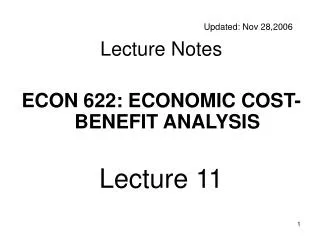
Updated: Nov 28,2006 Lecture Notes ECON 622: ECONOMIC COST-BENEFIT ANALYSIS Lecture 11. COSTS AND BENEFITS OF ELECTRICITY INVESTMENTS. Economic Valuation of Additional Electricity Supply. Willingness to pay for new connections Willingness to pay for more reliable service

E N D
Updated: Nov 28,2006 Lecture Notes ECON 622: ECONOMIC COST-BENEFIT ANALYSIS Lecture 11
Economic Valuation of Additional Electricity Supply • Willingness to pay for new connections • Willingness to pay for more reliable service • Resource cost savings from replacement of more expensive generation plants
$ S D 0 PMAX=P’ B C P0m F D0 0 Q’ Quantity Q0 ECONOMIC VALUE OF ELECTRICITY FOR NEW CONNECTIONS OR FOR REDUCTION OF WITH ROTATING POWER SHORTAGES Shaded area = economic value of shortage power (Q’-Q0) = Power shortage, evenly rotated to all customers Assuming willingness to pay (WTP) of all customers are also evenly distributed from highest 0P’ to lowest P0m: Economic Value of Additional Power Supply = ((PMAX+ P0m)/2) * (Q’-Q0)
D S0 P’ B C Pt F D0 0 Q0 Quantity Q’ ECONOMIC VALUE OF ELECTRICITY COMPUTATION FORMULA P’ = Maximum willingness to pay per unit of shortage power = 2 (capital costs of own generation/KWh) + Fuel Costs/KWh Need one generation to produce electricity and the second generation to provide reliability
WILLINGNESS TO PAY (WTP) FOR SHORTAGE POWER IN INDIA Customer Class Highest WTP* 1996 Rs/kwh COMMERCIAL 4.00 (Diesel autogeneration) INDUSTRIAL 3.22 (Diesel autogeneration) FARMER 3.77 (Diesel pump replacement) RESIDENTIAL 10.00 (Kerosene replacement) • Based on the financial costs of autogeneration or fuel replacement, World Bank Report, 14298-IN, 1996, for Orissa state of India. Actual WTP should be higher because of the inconveniences of operating diesel generators, diesel pumps, kerosene lamps and burners.
OWN-GENERATION COST AND WILLINGNESS TO PAY IN MEXICO Total Own-generation Cost ($/kWh) 0.169 Average Power Price (Gross of Tax, $/kWh) 0.037 Maximum Willingness To Pay ($/kWh) 0.212 Average Willingness To Pay ($/kWh) 0.125
Estimated Cost of Power Failure • 1. Based on willingness to pay • Based on customers survey • 2. Based on actual costs to users • 3. Based on linear relationship between GDP and electricity consumption of industrial/commercial users
Estimated Cost of Power Failure* • 1. Based on Willingness to Pay • Based on customers survey (Contingent valuation) • Ontario Hydro Estimates of Outage Costs (1981 US$/kwh) • Duration Large Small Commercial Residential • Manufacturers Manufacturers • 1 min 58.76 83.25 1.96 0.17 • 20 min 8.81 13.56 1.66 0.15 • 1 hr 4.35 7.16 1.68 0.05 • 2 hr 3.75 7.35 2.52 0.03 • 4 hr 1.87 8.13 2.10 0.03 • 8 hr 1.80 6.42 1.89 0.02 • 16 hr 1.45 4.96 1.75 0.02 • Average** 2.15 6.38 1.98 0.12 • All groups average***: 1.96 • Average power price: 0.025 • Average willingness for power during outage = 78.4 times average power price. • English Estimate (1996): 4 $/kwh • * C.W. Gellings and J.H. Chamberlin, Demand-Side Management: Concepts and Methods, Liburn, Georgia, The Fairmont Press, Inc., 1988. • ** Based on system simulation model • *** Based on shares: 13.5/13.5/39/34 %.
COST OF POWER FAILURE IN NEPAL* (Multiples of electric tariff) Year 1 2 3 4 5 Firm 1 5.56 2.73 5.01 1.50 3.43 Firm 2 3.31 2.86 1.71 3.24 3.76 Firm 3 15.25 11.77 14.37 12.16 5.26 Average each year 8.04 5.79 7.03 5.63 4.15 Average all years 6.13 Estimated Cost of Power Failure(continued) 2. Based on actual costs to users (Loss in contribution to profits) * Source: Table 7-10, Roop Jyoti, Investment Appraisal of Management Strategies for Addressing Uncertainties in Power Supply in the Context of Nepalese Manufacturing Enterprises, PhD Thesis, The Kennedy School of Government, Harvard University,December, 1998.
Estimated Cost of Power Failure(continued) San Diego (sudden outage of a few hours)* (1981 US $/kwh) Industrial Commercial Direct User 2.79 2.40 Employees of Direct User 0.21 0.09 Indirect User 0.12 0.13 Total 3.12 2.62 Multiples of Av Tariff** 62.4 52.4 Key West, Florida (rotating blackout for 26 days)* % of Cost Multiples Time of Price Nonresidential Users 4.8 $2.30/kwh 46.0 * Electric Power Research Institute study EPRI EA-1215, 1981, Vol. 2. ** Average price in 1981 is 0.05 $/kwh.
Estimated Cost of Power Failure (continued) 3. Based on linear relationship between GDP and electricity consumption of industrial/commercial users* Outage cost = 1.35 (1981$/kwh) Or: = 27 (multiples of the average power price) * M. L. Telson, “The Economics of Alternative Levels of Reliability for Electric Power Generation Systems,” Bell Journal of Economics, Autumn, 1975.
Summary: Average power outage cost ranges from 6 to 80 times of the average power price.
Load Curve hours for Year Load Duration Curve hours for Year Capacity MW Capacity MW 8760 hrs Peak hours Off-Peak hours 8760 hrs
Calculation of Marginal Cost of Electricity Supply • During the off-peak hours when the capacity is not fully utilized, the marginal cost in any given hour is the marginal running cost (fuel and operating cost per Kwh) of the most expensive plant operating during that hour. • During the peak hours, when generation capacity is fully utilized, the marginal cost of electricity per Kwh is equal to the marginal running cost of the most expensive plant running at the time plus the capital costs of adding more generation capacity, expressed as a cost per Kwh of peak energy supplied.
Optimal Stacking of Thermal Capacity KwH MC4=0.08+ 400(0.15)/1000=0.14/KWH 1 MC3=0.05/KWH 2 MC2=0.04/KWH 3 4 MC1=0.03/KWH H2 H3 H4 1000 1500 4500 H4 solve for the minimum number of hours to run a plant 4 or the maximum number to run plant 3. v = r+ d =0.15 v(K4)+f4(H4)=v(K3)+f3(H4) 0.15(1000)+0.03(H4)=0.15(700)+0.04(H4) (150-105)=0.4(H4)-0.03(H4) 45=0.01H4 H4=4500
Annualized Cost of Generation Investments Contribution to Generation Investments CapitalAnnual CostvCost Plant 1: 400 * 0.15 = 60 Plant 2: 600 * 0.15 = 90 Plant 3: 700 * 0.15 = 105 Plant 4: 1000 * 0.15 = 150 Total capital cost of system $405 per year. HoursPriceMCAmount $/yr. Plant 1: 1000 * (0.14 – 0.08) = 60 Plant 2: 1000 * (0.14 – 0.05) = 90 Plant 3: 1000 * (0.14 – 0.04) = 100 Plant 4: 1000 * (0.14 – 0.03) = 110 Plant 3: 500 * (0.05 – 0.04) = 5 Plant 4: 500 * (0.05 – 0.03) = 10 Plant 4: 3000 * (0.04 – 0.03) = 30 Total contribution per year = $405 Plant 1 60 60 90 90 Plant 2 105 Plant 3 5 100 Plant 4 150 110 10 30 Total: $ 405 1000 1500 4500
Stacking Problem: when do we replace a thermal plant? KW Output of plant #5 that substitutes for plant #1 = Q1 Hydro storage Output of plant #5 that substitutes for plant #2 = Q2 H1 1 (2) Output of plant #5 that substitutes for plant #3 = Q3 2 (3) H2 Output of plant #5 that substitutes for plant #4 = Q4 H3 3 (4) H4 4 (5) Load curve for plants 2,3,4 after 5 is introduced The question is whether or not we should build plant #5. We use the most efficient plant first and then use the next most efficient and so on until the least efficient we need to meet demand. • Assume plant #5 has equal capacity to each of the other plants we would then have to shift all of the plants up one stage in production, thus there is no need to use plant number one now. • Benefits to Plant #5: It is going to be producing most of the time. Part of the time 5 is effectively substituting for 4, part for 3, part for 2, and part for 1.
Two approaches to calculating benefits A. The new plant is used to substitute for part of the other plants that now do not produce as much as previously: Benefits Q4 x (0.03 – 0.02) Q3 x (0.04 – 0.02) Q2 x (0.05 – 0.02) Q1 x (0.08 – 0.02) Total A B. Alternative approach • Let H1, H2, H3, H4, be amount of electricity previously produced by plants 1 to 4. Original Total Cost New Total Cost H4 x 0.03 H4 x 0.02 H3 x 0.04 H3 x 0.03 H2 x 0.05 H2 x 0.04 H1 x 0.08H1 x 0.05 Total B Total C Total A = Total B -Total C. • We now compare total A with the annual capital cost of plant 5.
The Situation where variations in the efficiency of thermal plants are taken into account The optimum price to charge at any hour is the marginal running cost of the oldest (least efficient) thermal plant that is in operation during that hour. In this case, the benefits attributable to an investment in new capacity turn out to be the savings in system costs that the investment makes possible; and the present value of expected benefits is C(k) - the marginal running cost of a plant built in year k H(k,t) - the number of kilowatt-hours in the production of which a new plant would substitute for plants built in year k C(j) – running cost of plant j
When the plant is new, it is generating benefits all the time, but as it ages, and is supplanted at the base of the system by more efficient plants, it generates benefits only part of the time.Given this, the key investment criterion can be represented quite simply if we assume that the function Declines exponentially through time at annual rate of y.
Marginal Cost Pricing of Electricity • Efficient pricing of electricity. The basic assumption that we make is that the demand for electricity is increasing over time, 5-10% each year. Therefore with existing capacity economic rents will increase over time.
Price of electricity • If choice is to either stay at A capacity forever, or to stay at B forever, then we add up the consumer surpluses between A and B to see if B plant is worthwhile to install. Growth of Economic Rent Over Time Dt2 Dt1 Dt0 0 A B Q Price of electricity • If we expand capacity from A to B to C in subsequent time period. Benefits of A Dt2 Benefits of B Dt1 Benefits of C Dt0 0 Q A B C
Load Curve for Hours of Day • We start with the assumption that all we have are homogeneous thermal plants. Capacity in K.W. K0 Qt1 Qt0 0 Hours of day • If demand increases to Qt1 we either ration the available electricity or we build more capacity.
Load Curve for Hours of Day Surcharge cents Capacity in K.W. • by varying the price of electricity through time we can spread out demand so that it does not exceed capacity. K0 4 Si = Surcharge 3 2 1 Qt0 0 0 Hours of day • It is possible to keep quantity demanded constant by varying the price with the use of a surcharge. • Let Ki be the length of time each surcharge is operative. Si is the difference between MC and the price charged, then: • It is the economic rent accruing to the existing capacity.
Example • A kilowatt is the measure of capacity. • 1 K.W. of capacity can produce 8760 Kilowatt hour (KWH) per year. • Assume it costs $400 /kw of capital cost, and the social opportunity cost of capital plus depreciation = 12%. Therefore we need $48 of rent per year before we install another additional k.w. of capacity. • As demand increases through time we require a higher surcharge in order to contain capacity. Price used to ration capacity. • This will generate more economic rent, and if this rent is big enough it would warrant an expansion of capacity. • The objective of pricing in this way is to have it reflect social opportunity cost or supply price. • In practical cases the price does not vary continuously with time but we have surcharges that go on and off at certain time periods.
Example (Cont’d) • The “Load Factor” = KWH generated/8760 kwh • Capital costs of per KW of capacity = 400/KW • 10% interest + 2% depr = $48/yr • Marginal running costs = 3 cents per KWH • Peak hours are 2400 out of the year • Off peak optimal charge is 3 cents per KWH • On peak optimal charge is 5 cents per KWH • Implicit rent of any new capacity = 2400 x 2 cents = $48/year
Choice of different types of Electricity Generation Technologies to make Electricity Generation System • Thermal Generation: • Nuclear • Large fossil fuel plants • Combined cycle plants • Gas turbines • Hydro Power • Run of the Stream • Daily Reservoir • Pump Storage
Thermal vs. Hydro Generation • The thermal capacity is relatively homogeneous if capacity costs are higher generally fuel costs are lower. e.g. Coal plant versus combined cycle plant. • With hydro storage or use of the stream every particular site is different. • Costs may range over a 5 fold difference.
Run of the Stream • No choice of when the water will come. • Water comes at a zero marginal cost, therefore should use it when it comes. • Suppose river runs for 8760 hrs. at full generation capacity. • We will assume that the highest potential output during the year of the run of the stream is always less than total demand. Some thermal is being used. • Peak hours = 2400 • Off peak hours = 6360 • Savings as compared to thermal plant (from previous example) • 2400 x 5¢ 120.00 Peak rationed price = 5 ¢ • 6360 x 3¢190.80 off peak MRC of thermal = 3 ¢ 310.80 per year Question: Is US$ 310.80 per year enough to pay for run of stream capital plus running costs?
Daily Reservoir • Constructed to meet the peak day hours. • To store water during the off peak for use during the peak hours. • We don't generate any more electricity but we use the same amount of water and use it to produce peak priced electricity i.e. (5¢) instead of off peak (3¢) electricity. • Instead of 2400 x 5 ¢ = $120.00 6360 x 3 ¢ = $190.80 = $310.80 • We get 8760 x 5 ¢ = $438.00. Net benefits = $127.20 • The costs are that of building the reservoir and the additional hydro generating capacity so as to generate more electricity in the peak hours.
Daily Reservoir (Cont’d) • If previous run of stream generated 100 KW for 24 hours, now we will generate 300 KW for 8 hours. • The gain from this switch in water is what we compare with the extra cost. • If we now produce off peak electricity with thermal instead of run-of-the stream then this opportunity cost is calculated when calculating the opportunity costs of the daily reservoir. • The additional marginal running costs of the thermal plants needed to meet the off peak demand are deducted from the benefits of switching off-peak run-of-stream water to peak time water.
Pump Storage • We use off peak electricity to pump water up to a high area so that it can be released to produce electricity during peak demand periods. Example: • It takes 1.4 KWH off peak to produce 1KWH on peak • Off peak value = 3 ¢ KWH Peak = 5 ¢ KWH • There is a profit here of [(5¢ - 3¢*1.4) = (5¢ - 4.2 ¢)] = 0.8 ¢/KWH of peak hour generated • Pump storage is becoming feasible because of the existence of nuclear and very large fossil fuel plants. • These plants are very costly to shut off and on. • Therefore, their surplus in off peak hours is very cheap electricity. • With large storage at top and bottom of till, a very small stream is all that is needed to produce a very large power station and use nuclear power to pump water back up on off peak hours.
Multipurpose Dams • Multipurpose dams are used for irrigation, power and flood control. • However, with multipurpose dams it is possible to have conflicting objectives. • For example, it may be the case that irrigation water is needed in summer, but electrical power is at its lowest demand in summer. • We may have to adjust prices of electricity to shift some of the demand to times when irrigation water is required. • The different objectives have to be weighted. • A useful solution is to provide the water during the peak time hours for electricity and then build a small regulatory dam to provide water for irrigation. • The conflicting objectives may cause us to not have any optimal strategy over the year, but we still may be able to maximize during the day. • In this case we still will have to have a larger thermal capacity than in the case of no irrigation objective.
How do we price for the peak if the alternative is thermal generation? Capacity Hydro • Assume quantity of water available is fixed. • With an increase in peak demand we have to increase the thermal capacity and it is based on this cost that we have to calculate the peak time surcharge. Hydro Thermal 2 Thermal 1 2400 4000 8760 hrs Suppose system peak = 2,400 hours Thermal peak = 4,000 hours • It is over the 4,000 hours that we spread the capital costs of new thermal plants. If $48/kw needed per year to cover the capital costs then we only require a surcharge of 1.2 ¢/Kwh (4800¢/4000hrs. = 1.2¢/Kwh) • To find the price that should be charged for electricity during the peak hours, we add the capacity charge of 1.2 ¢ to the costs marginal running cost of the least efficient thermal plant operating during these hours. • As long as we peak with hydro storage then the benefit of increasing hydro is the thermal peak cost.