Download
1 / 31
310 likes | 459 Views
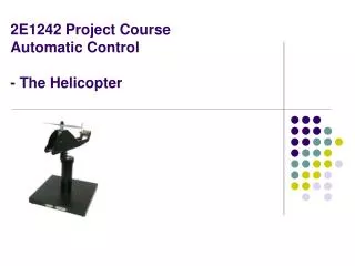
2E1242 Project Course Automatic Control - The Helicopter. The team. David Höök Henric Jöngren Pontus Olsson Ksenija Orlovskaya Vivek Sharma. Resources. Helicopter with two degrees of freedom (Humusoft) Input voltage to two DC motors driving the main and tail propellers (MIMO-system)

E N D
The team • David Höök • Henric Jöngren • Pontus Olsson • Ksenija Orlovskaya • Vivek Sharma
Resources • Helicopter with two degrees of freedom (Humusoft) • Input voltage to two DC motors driving the main and tail propellers (MIMO-system) • Output horisontal and vertical angles • Labview (communicating with process) • Matlab (simulation, model validation)
The challenge • MIMO system under influence of cross-coupling • Modelling • Many non directly measurable parameters • Subsystems interlinked through many parameters
Main objective The helicopter is supposed to: • Follow a prespecified trajectory that illustrates its performance limitations • Attenuate external disturbances • Hair-drier simulating hard wind • Change of mass centre - adding a load to helicopter
Modelling Helicopter divided into subsystems • Main motor and vertical movement • Tail motor and horisontal movement Cross coupling: • Main motor to horisontal movement (reaction torque) • Horisontal movement to vertical movement (gyroscopic moment) • Cross coupling from tail motor reaction to vertical moment and vertical gyro effects neglected.
Modelling Main motor and vertical movement
Modelling Tail motor and horisontal movement
Modelling Physically derived differential equation model
Modelling Black box • First approach • subsystem and model are compared
Modelling White box / Grey box • Measure parameters corresponding to the physical model. • Weight, distances • Determine non directly measurable parameters • Frictions, inertias, gyro, reaction torque – iteratively by adjusting parameters from model to fit responses from process ’ • Time constants for motor dynamics • Adjusting curves to static measurement data • Functions mapping insignals to pull force, rotor velocity and reaction torque
Validation, vertical movement Step response of verticalmovement in model and process t
Validation, horisontal movement Step response of horisontal movement in model and process t
Validation, reaction torque Response in horisontal movement from step in main motor t t
Validation, gyroscopic effect Response in vertical movement from step in tail motor t
Validation, total model • System too unstable to be validated open-loop • Two manually tuned PID-controllers are used Model Process
Modelling Conclusion – what have we learned about modelling? • More difficult than expected • Dependent system • Tuning a parameter of one subsystem will affect the behavior of other subsystems. • Must find good balance between the best approximation of the separate subsystems and the performance of the total system. • When is the model good enough? – When it is fulfilling its purpose • White box: more insight and understanding of system than Black box • Black box: less time consuming than white box
Control Different controllers • Manually adjusted PID – one for each degree of freedom • LQ controller with observer – one for the total system Is it necessary to spend weeks modelling if a quickly tuned P.I.D. can solve the control problem? -The manually adjusted PID against the model dependent LQ…
Control Introducing cross gain – elimination of cross coupling u_vert(t) y_vert(t) e_vert(t) r_vert(t) + G_vert PID_vert - Cross gain sK1 K2 r_hor(t) e_hor(t) + + G_hor PID_hor - u_horizontal(t) y_hor(t) Conclusion…
Validation, vertical movement Step response of verticalmovement in model and process t
r(t) u(t) y(t) Fr + Helicopter -L Observer Control LQ with observer - Not all states measureable - introducing state observer
Control • Model linearized by hand • Equilibrium point taken from real process (input voltages and angles) White noise with intensities: :No covariance between the noise :Design variables
Control Singular values
Control LQ PID
Control Conclusion – what have we learned about control? • Different regulators: PID, LQ ,close look at advantages and disadvantages over each other. • The functions are fulfilling their purposes.
THE END… 11/5 kl. 03.12