Download
1 / 62
620 likes | 759 Views
Variability in the ocean - from modewater biogeochemistry to SST. Holger Brix UCLA, JIFRESSE and Dept. of Atmospheric and Oceanic Sciences JPL, 16 September 2008. Acknowledgements. Curtis Deutsch, UCLA Nicolas Gruber, ETH, Z ürich Scott Doney, Ivan Lima, WHOI

E N D
Variability in the ocean - from modewater biogeochemistry to SST Holger Brix UCLA, JIFRESSE and Dept. of Atmospheric and Oceanic Sciences JPL, 16 September 2008
Acknowledgements • Curtis Deutsch, UCLA • Nicolas Gruber, ETH, Zürich • Scott Doney, Ivan Lima, WHOI • Crews and scientists of NOAA, UH, BBSR, and other research vessels • Dimitris Menemenlis, JPL
Outline • Mode water biogeochemistry • Global Carbon Cycle Perturbations • Carbon and the Ocean • Why mode waters (and what are they anyway)? • Mode water variability - time-scales and places • Modeling the gaps • Sea surface temperatures and heat flux variability in ECCO2 and beyond
Outline • Mode water biogeochemistry • Global Carbon Cycle Perturbations • Carbon and the Ocean • Why mode waters (and what are they anyway)? • Mode water variability - time-scales and places • Modeling the gaps • Sea surface temperatures and heat flux variability in ECCO2 and beyond
The Global Carbon Cycle Sarmiento & Gruber, 2002
Perturbation of Global Carbon Budget (1850-2006) 2000-2006 deforestation Source tropics extra-tropics 1.5 CO2 flux (Pg C y-1) Sink Time (y) Le Quéré, unpublished; Canadell et al. 2007, PNAS
Perturbation of Global Carbon Budget (1850-2006) 2000-2006 fossil fuel emissions 7.6 Source deforestation 1.5 CO2 flux (Pg C y-1) Sink Time (y) Le Quéré, unpublished; Canadell et al. 2007, PNAS
Perturbation of Global Carbon Budget (1850-2006) 2000-2006 fossil fuel emissions 7.6 Source deforestation 1.5 CO2 flux (Pg C y-1) Sink Time (y) Le Quéré, unpublished; Canadell et al. 2007, PNAS
Perturbation of Global Carbon Budget (1850-2006) 2000-2006 fossil fuel emissions 7.6 Source deforestation 1.5 CO2 flux (Pg C y-1) atmospheric CO2 4.1 Sink Time (y) Le Quéré, unpublished; Canadell et al. 2007, PNAS
Perturbation of Global Carbon Budget (1850-2006) 2000-2006 fossil fuel emissions 7.6 Source deforestation 1.5 CO2 flux (Pg C y-1) atmospheric CO2 4.1 Sink ocean 2.2 Time (y) Le Quéré, unpublished; Canadell et al. 2007, PNAS
Perturbation of Global Carbon Budget (1850-2006) 2000-2006 fossil fuel emissions 7.6 Source deforestation 1.5 CO2 flux (Pg C y-1) atmospheric CO2 4.1 Sink land 2.8 ocean 2.2 Time (y) Le Quéré, unpublished; Canadell et al. 2007, PNAS
Outline • Mode water biogeochemistry • Global Carbon Cycle Perturbations • Carbon and the Ocean • Why mode waters (and what are they anyway)? • Mode water variability - time-scales and places • Modeling the gaps • Sea surface temperatures and heat flux variability in ECCO2 and beyond
The Biogeochemical loop N. Gruber, 2002
Marine Phytoplankton http://www.amonline.net.au/exhibitions/beyond/phytoplnkton/ From top left: Diatoms, Radiolaria, Dinoflagellates
The Biogeochemical loop Production Export N. Gruber, 2002
Production, Respiration, Export Photosynthesis “Net Primary Production (NPP)” Corg CO2 NPP Phytopl. Bacteria Zoopl. Rh Export Production Respiration (Heterotrophic) Net Community Production: NCP = NPP - Rh
The Biogeochemical loop Production NPP Export (=NCP) N. Gruber, 2002
NPP-NCP-POC at HOT(Hawaii Ocean Time-Series) POC: Particulate Organic Carbon Brix et al., 2006
Spatial patterns in ∆pCO2 due to biology and temperature are also mostly opposing each other!
Anthropogenic CO2 Gruber (2002)
Outline • Mode water biogeochemistry • Global Carbon Cycle Perturbations • Carbon and the Ocean • Why mode waters (and what are they anyway)? • Mode water variability - time-scales and places • Modeling the gaps • Sea surface temperatures and heat flux variability in ECCO2 and beyond
Surface density, isopycnal outcrops Waters will move mostly along surfaces of constant density.
What Are Mode Waters? Definitions after Hanawa and Talley (2001) • Homogeneity of water properties (such as temperature, salinity, oxygen) • Thickening of isopycnal layer - substantial volume • At a single vertical profile, mode water appears as low vertical density gradient (pycnostad) between high gradients (seasonal and main pycnocline) • Mode water is found well beyond its outcropping areas as a result of advection • Formation or maintenance usually associated with wintertime convective mixing
Mode Waters Example: 18o Mode Water Subtropical Mode Water (STMW) in the North Atlantic Potential Temperature
Why are we interested in Mode Waters? • Mode waters can take up anthropogenic CO2 and hide it from the atmosphere (buffer capacity) • After a time delay (years to decades) mode waters re-emerge at (possibly distant) regions And where do we find them? • In all ocean basins • “Descending” on isopycnals from outcrop regions
Mode Waters Talley, 1999
Intermediate Waters LSW NPIW AAIW Talley, 1999
Outline • Mode water biogeochemistry • Global Carbon Cycle Perturbations • Carbon and the Ocean • Why mode waters (and what are they anyway)? • Mode water variability - time-scales and places • Modeling the gaps • Sea surface temperatures and heat flux variability in ECCO2 and beyond
DIC at BATS (Bermuda) Bates et al., 2001
Chlorophyll in the NAtl. Lévy, 2005; Palter et al., 2005
Apparent Oxygen Utilization AOU = O2,SAT - O2 (measure of respiration) Figure prepared by Niki Gruber
AAIW MED SPMW LAB NADW AOU = [O2sat] - [O2] APPARENT OXYGEN UTILIZATION STMW SPMW AAIW MED Johnson & Gruber, Prog. Oceanography, 2007 LAB NADW
AOU CHANGES 2003-1993 Johnson & Gruber, Prog. Oceanography, 2007
AOU AND DIC CHANGES 2003-1993 Expected change from anthropogenic CO2: max 0-8 mmol/kg Johnson & Gruber, Prog. Oceanography, 2007
O2 anomaly at HOT (Hawaii) Deutsch, 2006
Observed AOU differences North Pacific Deutsch et al. (2006)
Outline • Mode water biogeochemistry • Global Carbon Cycle Perturbations • Carbon and the Ocean • Why mode waters (and what are they anyway)? • Mode water variability - time-scales and places • Modeling the gaps • Sea surface temperatures and heat flux variability in ECCO2 and beyond
Modeled AOU differences North Pacific Deutsch et al. (2006)
Components of Variability Changes in AOU can be decomposed into components: AOU = AOUbiol + AOUvent + AOUcirc Using: Multiple simulations with climatological OUR (OUR = dAOU/dt) and/or preformed climatological AOU fields
O2 change, 1990’s-1980’s, = 26.6Deutsch et al. (2006) Total Circulation Ventilation Biology
Origin of O2 anomalies1990s - 1980s a,b: ventilation c,d: circulation a,d: decadal trends b,c: interannual perturbations a b c d Deutsch et al. (2006)