Download
1 / 30
300 likes | 451 Views
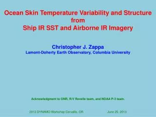
Ocean Skin Temperature Variability and Structure from Ship IR SST and Airborne IR Imagery. Christopher J. Zappa Lamont-Doherty Earth Observatory, Columbia University. Acknowledgment to ONR, R/V Revelle team, and NOAA P-3 team. 2013 DYNAMO Workshop Corvallis, OR June 25, 2013. Data QC.

E N D
Ocean Skin Temperature Variability and Structure from Ship IR SST and Airborne IR Imagery Christopher J. Zappa Lamont-Doherty Earth Observatory, Columbia University Acknowledgment to ONR, R/V Revelle team, and NOAA P-3 team. 2013 DYNAMO Workshop Corvallis, ORJune 25, 2013
Data QC • R/V Revelle • Up and Down-looking LW Infrared Radiometers • Provides continuous Skin Temperature Measurement for Legs 2, 3, and 4. • Ready and available to community
Skin Temperature Importance for Bulk Flux Tskin (SST) (= KT15 Tskin); Tbulk (= Tsnake); Tcool_layer (= Tsnake- calculated cool layer correction)
Data QC • P-3 • Down-looking LW Infrared Cameras (240 x 320 and 640 x 512) • IR cameras has sensitivity of 0.02 K • Important corrections are required for accurate skin temperature estimates • Down-looking Visible Cameras (5 MP: 2000 x 2500; 1 MP: 1000 x 1000) • Resolution depends on altitude • 0.5 to 3.0 m resolution in IR • 0.1 to 0.6 m resolution for Visible
Foci • Response of the Ocean Surface to Convective Events • Observed significant differences in the structure of the ocean surface during convective events at different phases of the MJO • Evolution of the sea surface patchiness and upper ocean structure during convective events • Have multiple instances to build up consistent picture • Evidence suggests that the sea surface patchiness quickly evolves from its initial state to a system dominated by LC as the convective front (precip / high winds) propagates over a specific location, to a system behind the convective front ( no precip / winds??) where the sea surface patchiness appears without the strong forcing • LC organizes the fresh water and then sea surface patchiness evolves after the water Slumps back • Related to fresh water lenses as well as sea surface patchiness • Measure the Scales of Coherent Structure to compare with MO Length scale • Evolution of the short fetch gravity wave field and wave breaking through the convective events • Have multiple instances to build up consistent picture • Evidence suggests that the wave breaking quickly develops across the convective front • No evidence to date of enhanced breaking ahead of the front • Crucial to know the convective front orientation and propagation direction (S-POL, P-3 Radars, Revelle Radars) • Evolution of the skin temperature structure as it advects towards the Revelle • Upper Ocean mixing in response to the atmospheric forcing • Use the combination of the Moum upper ocean temperature structure at the Revelle and the propagated Airborne SST structure to understand the mixing of fresh precipitation • Initial simple test shows evolution of temperature structure. • Measure the Scales of Coherent Structure to compare with MO Length scale
Onset Equatorial Convection MJO 2 Strong winds in a moist environment 0512Z B A 0514Z Red line: Aircraft track Red Dots: Mosaic Imagery Black line: Vertical cross section Black dot: Dropsonde location Nov 22 – Northern ITCZ 1st RCE
Onset Equatorial Convection MJO 2 Strong winds in a moist environment • Large-Scale Temperature change of up to 1.0°C across the front
Onset Equatorial Convection MJO 2 Strong winds in a moist environment 0512Z B A 0514Z Red line: Aircraft track Red Dots: Mosaic Imagery Black line: Vertical cross section Black dot: Dropsonde location Nov 22 – Northern ITCZ 1st RCE
Onset Equatorial Convection MJO 2 Strong winds in a moist environment • Small-scale temperature variability of 0.1°C m-1 with horizontal wind row scales of O(10-50) m • Small-scale temperature variability of 0.2°C m-1 with horizontal patchiness scales of O(10-50) m
Onset Equatorial Convection MJO 2 Strong winds in a moist environment • Small-scale temperature variability of 0.1°C m-1 with horizontal wind row scales of O(10-50) m • Small-scale temperature variability of 0.2°C m-1 with horizontal patchiness scales of O(10-50) m
Foci • Response of the Ocean Surface to Convective Events • Observed significant differences in the structure of the ocean surface during convective events at different phases of the MJO • Evolution of the sea surface patchiness and upper ocean structure during convective events • Have multiple instances to build up consistent picture • Evidence suggests that the sea surface patchiness quickly evolves from its initial state to a system dominated by LC as the convective front (precip / high winds) propagates over a specific location, to a system behind the convective front ( no precip / winds??) where the sea surface patchiness appears without the strong forcing • LC organizes the fresh water and then sea surface patchiness evolves after the water Slumps back • Related to fresh water lenses as well as sea surface patchiness • Measure the Scales of Coherent Structure to compare with MO Length scale • Evolution of the short fetch gravity wave field and wave breaking through the convective events • Have multiple instances to build up consistent picture • Evidence suggests that the wave breaking quickly develops across the convective front • No evidence to date of enhanced breaking ahead of the front • Crucial to know the convective front orientation and propagation direction (S-POL, P-3 Radars, Revelle Radars) • Evolution of the skin temperature structure as it advects towards the Revelle • Upper Ocean mixing in response to the atmospheric forcing • Use the combination of the Moum upper ocean temperature structure at the Revelle and the propagated Airborne SST structure to understand the mixing of fresh precipitation • Initial simple test shows evolution of temperature structure. • Measure the Scales of Coherent Structure to compare with MO Length scale
Wave Breaking during Convection Strong winds in a moist environment A B Nov 24–Active Phase Band 1st RCE 0456Z 0450Z B A
Wave Breaking during Convection Strong winds in a moist environment Breaking crest length distributions. Note that the wave age (cp/u*) plays a significant role in breaking. The dashed line represents the cb-6 dependence predicted by Phillips [1985]. • Wave Breaking is strong along the front yet diminished behind.
Foci • Response of the Ocean Surface to Convective Events • Observed significant differences in the structure of the ocean surface during convective events at different phases of the MJO • Evolution of the sea surface patchiness and upper ocean structure during convective events • Have multiple instances to build up consistent picture • Evidence suggests that the sea surface patchiness quickly evolves from its initial state to a system dominated by LC as the convective front (precip / high winds) propagates over a specific location, to a system behind the convective front ( no precip / winds??) where the sea surface patchiness appears without the strong forcing • LC organizes the fresh water and then sea surface patchiness evolves after the water Slumps back • Related to fresh water lenses as well as sea surface patchiness • Measure the Scales of Coherent Structure to compare with MO Length scale • Evolution of the short fetch gravity wave field and wave breaking through the convective events • Have multiple instances to build up consistent picture • Evidence suggests that the wave breaking quickly develops across the convective front • No evidence to date of enhanced breaking ahead of the front • Crucial to know the convective front orientation and propagation direction (S-POL, P-3 Radars, Revelle Radars) • Evolution of the skin temperature structure as it advects towards the Revelle • Upper Ocean mixing in response to the atmospheric forcing • Use the combination of the Moum upper ocean temperature structure at the Revelle and the propagated Airborne SST structure to understand the mixing of fresh precipitation • Initial simple test shows evolution of temperature structure. • Measure the Scales of Coherent Structure to compare with MO Length scale
Comparison with Revelle in MJO 2 Strong winds in a moist environment • Use the combination of the Moum upper ocean temperature structure at the Revelle and the propagated Airborne SST structure to understand the mixing of fresh precipitation.
Suppressed Phase of MJO Strong gradient in convection between ITCZ and Equator. Weak winds and dry near Gan. • Small-scale temperature variability of 0.1°C m-1 with muted and smoothed horizontal scales • Large-scale temperature fronts associated with fresh convective event of 0.5°C
Fig D3. Composite of all103 identified rain events, showing the response of air temperature, U10 relative to the surface currents, bulk water temperature, and SSTskin. The time for each event has been shifted to zero and then normalized by t*SST. Each variable has been zeroed by its value at the beginning of the rain event (the mean value of the 3 minutes prior for SSTskin). The mean ΔSST due to rain is 0.51˚C (attenuated here due to bin averaging). Fig D1. Histograms of the SSTskin response; the time to the maximum SST response , t*SST; cumulative rain for an event; length of rain event, Lrain; and time to peak rain rate, t*rain. A few very long events (> 10 hours) occur, but identified events are primarily about an hour long and deposit around 15 mm rain. • Distribution of stations within Terra Nova Bay, 1958-2004 Fig D2. Relationship between delta SSTskin (top row) and time to reach maximum ΔSSTskin, t*SST, (bottom row) with cumulative rain deposited; maximum rain rate; length of rain event; and time to reach maximum rain rate, t*rain; t*SST scales well to the length of the rain event and t*rain, suggesting that the distribution of rain rate is essentially Guassian within a rain event.
Actual MJO Stages A B C Conceptual moistening drying drying slow moistening moistening drying
Revelle in Visible and Infrared ??? ???