Download
1 / 22
220 likes | 310 Views
Explore the use of survival models incorporating macroeconomic data for accurate projections of credit default rates under adverse economic scenarios. Learn the model structure, estimation methods, and forecasting techniques for stress testing portfolios.

E N D
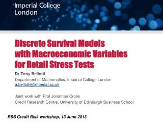
Discrete Survival Models with Macroeconomic Variables for Retail Stress Tests Dr Tony Bellotti Department of Mathematics, Imperial College London a.bellotti@imperial.ac.uk Joint work with Prof Jonathan Crook Credit Research Centre, University of Edinburgh Business School RSS Credit Risk workshop, 13 June 2013
Outline of this presentation Motivation. Model structure for including macroeconomic data. Forecasting using the model. Scenario stress testing of a portfolio using the model. Stress tests based on Monte Carlo simulation. Conclusion.
Motivation – Models for stress testing Stress testing requires a projection of income for a financial institution based on hypothetical adverse economic conditions. The adverse conditions may be provided as economic scenarios by regulatory bodies or may be generated internally. The projections of income are based partly on aggregation of projected losses on loan portfolios. Therefore there is a need for statistical/econometric models for different loan types which can be used to accurately project possible losses conditional on different economic scenarios.
Motivation – Survival models Why survival models? Natural to model time to default; Inclusion of dynamic data: behavioural and economic; Calculation of expected profit over the lifetime of loans. Why include macroeconomic variables? Build models that are sensitive to changes in the economy. Forecast default rates and expected losses more accurately. Stress test using statistical modelsallowing the inclusion of economic scenarios.
Discrete survival model of credit default The discrete survival model covers most options required of a dynamic credit risk model, whilst being computationally efficient. The following types of variables can be included: • Static variables about obigor (ie application or bureau data). • Duration (age of account) effect. • Vintage effects. • Behavioural variables (BVs) about credit usage and repayments. • Macroeconomic variables (MVs). • Frailty term (ie unknown account-level effect). • Unknown systemic (calendar time) effect.
Model structure where
Model estimation This is a panel model structure over accounts and duration . Need to specify a link function . This could be logit or probit. • Taking to be complementary log-log, ie , yields a discrete version of the Cox proportional hazard model. Most of the variables are included as fixed effect terms. Frailty and systematic effect are included as random effect terms, assumed to be normally distributed. Maximum marginal likelihood can be used to estimate coefficients on fixed effects () and variance of the random effects.
Using the model: Forecasts For forecasts, we may be interested in computing the probability of default (PD) within some time of opening an account: At aggregate (portfolio) level we are interested in expected value of default rate (DR) at some calendar time period : where is the number of accounts such that .
Using the model: Forecasting and stress testing Notice that for DR estimates, even if coefficient estimates on macroeconomic variables are small, they may have large overall effect because they are affecting all accounts in the same way at the same (calendar) time. Because the PD and DR are estimated as functions of macroeconomic variables, the essence of stress testing is to use values of these variables corresponding to recession scenarios to adjust the forecasts. Stress testing using scenarios then gives a point estimate adjustment. Generating economic simulations from a distribution of plausible future economic conditions, enables a distribution of estimates for PD and DR.
Illustration of scenario stress test Suppose we want to stress test PD on a UK credit card portfolio. Include several AVs and BVs. Include two MVs: UK interest rates (IR) and unemployment rate (UR) in millions, as differences over 12 months. Build a discrete survival model with logit link function. Estimate coefficients on IR and UR as 0.11 and 0.67 respectively (note, these figures are based on real model results). Suppose a log-odds score for a customer during “normal” conditions (IR=0 and UR=0) is -5.45. Then suppose a stress scenario #1: IR=+1.5 and UR=+0.25. And worse scenario #2: IR=+3 and UR=+1. How do the stressed scenarios affect the estimate of PD over a yearly period?
Example of scenario stress test Simplified version of calculation of stressed PD for illustration…. Therefore, stressed conditions (#1) represents an increase in PD of almost 38%.
Some issues for including variables in the model Behavioural variables (BVs) should have long lags (eg a year) to enable forecasting ahead. Macroeconomic variables (MVs) do not necessarily require long lags since macroeconomic models can be used to forecast ahead (eg GDP forecast models). BVs and MVs: Possibly include as aggregates (egmean, max, min or geometric lag). Trends in MVs: Use differences; eg growth in GDP instead of GDP. Correlations amongst MVs….
Correlation amongst macroeconomic variables We expect MVs to be highly correlated. This could lead to problems with the model estimation (multicollinearity). Two tactics to deal with this: • Variable selection: Hope to remove highly correlated variables. • Problem: This method is somewhat crude. • Factor analysis: Reduce MVs to orthogonal components. Factor analysis (eg PCA) Component 1: Component 2: Macroeconomic “factors” “Raw” MV time series • Example: Chicago Fed economic index (CFNAI).
Model over the business cycle / population drift Train over a whole business cycle, if possible, to get good estimates for MVs. • How much of the business cycle is needed? 5 years? • Explore breakpoints in the economy and effect on the model. Dealing with old data and population drift in the credit risk model. • That is, the MV estimate may require several years of data, whereas a useful default model may use just one year. • Possible solution: Two-part model… • Build long-term model with MV estimates; • Build default model on short amount of recent data; • Merge the two.
Result 1: Including MVs We now present some results using the discrete survival model for forecasting DR, stress testing and asset correlation estimates. UK credit card data covering a period from 1996 to mid-2006: • Training data 1996 to 2004 (over 400,000 accounts); • Out-of-sample test data 2005 to mid-2006 (over 150,000 accounts). Includes application variables (AVs), behavioural variables (BVs) and several macroeconomic variables (MVs). Two MVs were found to be statistically significant at 5% level: These results will be published soon in the International Journal of Forecasting.
Results 2: Forecasting DR (reality check) • Three alternative models are built with different variables to test forecasts of default rates (DR). • The mean absolute difference (MAD) between estimated an observed DR on the test data set is used as a performance measure. • The model with MVs gives the best result with lowest MAD. • This result is consistent across the test set over time.
Median Observed DR VaR (99% level) Expected shortfall (99% level) 0.5 0.75 1 1.25 1.5 1.75 2 2.4 Estimated default rate Region of expected shortfall calculation (99% level) (as ratio of median value) Result 3: Stress testing using simulation Monte Carlo simulation based on drawing economic scenarios from a plausible distribution of MVs. • VaR (99%) = 1.59 times median. • Expected shortfall (99%) = 1.73 times median.
Schema for stress test simulation method Test data set Monte Carlo simulation To compute Value at Risk and Expected shortfall Distribution over MVs Credit risk Model with MVs Random draws Loss distribution Compute DR / losses Value at Risk, and Expected shortfall
Stress testing by simulation Estimate macroeconomic distribution (MD) using historical values of MVs. Draw scenarios from the MD: • Normalization and Choleskydecomposition (to deal with collinearity between MVs). Extreme but plausible events. Including other elements in the simulation: • Random effects at account (estimates) and calendar time levels (draw from random effect distribution). • Model uncertainty (ie uncertainty in coefficient estimates).
Conclusion The discrete survival model with random effects is a rich model that allows us to consider a variety of important risk factors over time. It is computationally efficient. Empirical evidence shows the model gives improved forecasts and plausible stress test results. Requires some careful thought and analysis regarding exactly how time varying variables are included in the model.
Future work and open problems • Two-part model to avoid the problem of population drift. • Further methodological work required on the statistical problem of stress testing using simulation. • Test the method on a variety of different credit data.
Discrete survival models for stress testing Joint work by Prof Jonathan Crook* and Dr Tony Bellotti** * Credit Research Centre, University of Edinburgh Business School ** Department of Mathematics, Imperial College London • Email: a.bellotti@imperial.ac.uk • Web page: www2.imperial.ac.uk/~abellott/