Discrete Random Variables
Discrete Random Variables. Introduction. In previous lectures we established a foundation of the probability theory; we applied the probability theory to some applications; w e covered combinatorial problems; w e studied Bayesian theorem. In this lecture


Discrete Random Variables
E N D
Presentation Transcript
Introduction • In previous lectures • we established a foundation of the probability theory; • we applied the probability theory to some applications; • we covered combinatorial problems; • we studied Bayesian theorem. • In this lecture • we will define and describe the random variables; • we will give a definition of probability mass function and probability distribution functions; • a number of discrete probability mass functions will be given. • Properties of probability mass and cumulative functions will be given.
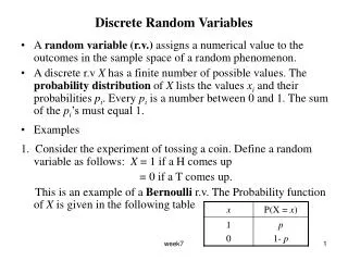
Definition of Discrete Random Variables • Sample space of a die is {1,2,3,4,5,6}, because each face of a die has a dot pattern containing 1,2,3,4,5, of 6 dots. • This type of experiment is called numerical valued random phenomenon. • What if outcomes of an experiment are nonnumerical? • The sample space of a coin toss is S = {tail, head}. It is often useful to assign numeric values to such experiments. Example: the total number of heads observed can be found as
Definition of Discrete Random Variables • The function that maps S into SX and which is denoted by X(.) is called a random variable. • The name random variable is a poor one in that the function X(.) is not random but a known one and usually one of our own choosing. • Example: In phase-shift keyed (PSK) digital system a ”0” or “1” is communicated to a receiver by sending • A 1 or a 0 occurs with equal probability so we model the choice of a bit as a fair coin tossing experiment. random variable
Definition of Discrete Random Variables • Random variable is a function that maps the sample space S into a subset of the real line. S SX • For a discrete random variable this subset is a finite or countable infinite set of points. • A discrete random variable may also map multiple elements of the sample space into the same number. One-to-one Many-to-one Example:
Probability of Discrete Random Variables • What is the probability P[X(si) = xi] for each ? • If X(.) maps each si into a different xi (or X(.)one-to-one), then because si and xi are just two different names for the same event • If, there multiple outcomes in S that map into the same value xi (X(.) is many-to-one) then sj’s are simple events in S and are therefore mutually exclusive. • The probability mass function (PMF) can be summarized as Random variable (RV) [] discrete RV The PMF is the probability that the RVX takes on the value xi for each possible xi.
Examples • Coin toss – one-to-one mapping • The experiment consists of a single coin toss with a probability of heads equal to p. The sample space is S = {head, tail} and the RV is • The PMF is therefore • Die toss – many-to-one mapping • The experiment consists of a single fair die toss. With a sample space of S = (1,2,3,4,5,6} and in interest only in whether the outcome is even or odd we define the RV as • The event is just the subset of S for which X(s) = xi holds.
Properties • Because PMFs pX[xi] are just new names for the probability P[X(s) =xi] they must satisfy the usual properties: • Property 1: Range values • Property 2: Sum of values If SX consists of M outcomes If SX is countably infinite. • We will omit the s argument of X to write pX[xi] = P[X = xi]. • Thus, we probability of event A defined on SX is given by
Example • Calculating probabilities based on the PMF • Consider a die with sides S = {side1, side2, side3, side4, side5, side6} whose sides have been labeled as with 1,2 or 3 dots. • Thus, • Assume we are interested in the probability that a 2 or 3 occurs or A = {2,3}, then
Important Probability Mass Functions • Bernoulli p =0.25 ~ is distributed according to • Binomial (M + 1)p max M = 10 p =0.25
Important Probability Mass Functions • Geometric p =0.25 • Poisson
Approximation of Binomial PMF by Poisson PMF • If in a binomial PMF, M ∞ as p 0 such that the product λ = Mpremains constant, then bin(M,p) Pois(λ) and λrepresents average number of successes in M Bernoulli trials. In other words, by keeping the average number of successes fixed but assuming more and more trials with smaller and smaller probabilities of success on each trial, leads to a Poisson PMF. M = 10 p =0.5 M = 100 p =0.05
Approximation of Binomial PMF by Poisson PMF • We have for the binomial PMF with p = λ/M 0 as M ∞. • For a fixed k,as M ,we have that and . • Using L’Hospital’s rule we have and therefore
Transformation of Discrete Random Variable • It is frequently of interest to be able to determine the PMF of the new random variable Y = g(X). • Consider a die which sides are labeled with the numbers 0,0,1,1,2,2. Then the transformation appears as many-to-one
Examples • In general, • Example: One-to-one transformation of Bernoulli random variable. • If X ~ Ber(p) and Y = 2X – 1, determine the PMF of Y. • The sample space SX = {0, 1} and consequently SY = {-1, 1}. It follows that x1 = 0 maps into y1 = -1 and x2 = 1 maps into y2 = 1. Thus, • Example: Many-to-one transformation • Let the transformation be Y = g(X) = X2 which is defined on the sample space SX = {-1, 0, 1} so that SY = {0, 1}. Clearly, g(xj) = xj2 = 0 only for xj = 0. • However, g(xj) = xj2 = 1 for xj = -1 and xj = 1. Thus, using (*) we have
Example: Many-to-one transformation of Poisson random variable • Consider X ~ Pois(λ) and define the transformation Y =g(X) as • To find the PMF for Y we use • We need only determine since . Thus, Taylor expansion
Cumulative Distribution Function • An alternative means of summarizing the probabilities of a discrete random variable is the cumulative distribution function (CDF). • The CDF for a RVX is defined as • Note that the value X = x is included in the interval. • Example: if X ~ Ber(p), then the PMF and the corresponding CDF are PMF CDF p = 0.25 p = 0.25
Example: CDF for geometric random variable • Since for k = 1,2,…, we have the CDF • Where [x] denotes the largest integer not exceeding x. • The PMF can be recovered from CDF by .
Example: CDF for geometric random variable • PMF and CDF are equivalent descriptions of the probability and can be used to find the probability of X being in an interval. • To determine for geometric RV we have • In general, the intervals (a,b] will have different from (a,b), [a, b), and [a,b] probabilities. • but
Properties of CDF • Property 3. CDF is between 0 and 1 • Proof: Since by def. FX(x) = P[X ≤ x] is a probability for all x, it must lie between 0 and 1. • Property 4. Limits of CDF as x -∞ and x ∞. • Proof: • since the values that X(s) can take on do not include -∞. Also • since the values that X(s) can take on are all included on the real line
Properties of CDF • Property 5. A monotonically increasing function g(.) is one in which for every x1 and x2 with x1≤ x2, it follows that g(x1) ≤ g(x2). • Proof: • Property 6. CDF is right-continuous • By right-continuous is meant, that as we approach the point x0 from the right, the limiting value of the CDF should be the value of the CDF at that point (definition) (Axiom 3) (def. and Axiom 1)
Properties of CDF • Property 7. Probability of interval found using the CDF • Proof: Since a < b and the intervals on the right-hand-side are disjoint, by Axiom 3 Or rearranging the terms we have that
Computer Simulations • Assume that X can take on values SX = {1,2,3} with PMF
Computer Simulations • u is a random variable whose values are equally likely to fall within the interval (0,1). It is called uniform RV. • To estimate the PMF a relative frequency interpretation of probability will yield • The CDF is estimated for all x via k = 1,2,3 M = 100 M = 100
Computer Simulations • Note that an inverse CDF is given by so we choose the value of x as shown below.
Exercise • Draw a picture depicting a mapping of the outcome of a clock hand that is randomly rotated with discrete steps 1 to 12. • Consider a random experiment for which S = {si : si = -3, -2, -1, 0, 1, 2, 3} and the outcomes are equally likely. If a random variable is defined as X(si) = si2, find Sx and the PMF.
Exercise • If X is a geometric RV with p =0.25, what is the probability that X ≥ 4? • Compare the PMFs for Pois(1) and bin(100, 0.01) RVs. • Generate realizations of a Pois(1) RV by using a binomial approximation. • Find and plot the CDF of Y = - X if X ~ Ber(1/4). pois
Homework problems • A horizontal bar of negligible weight is loaded with three weights as shown in Figure. Assuming that the weights are concentrated at their center locations, plot the total mass of the bar starting at the left (where x = 0 meters) to any point on the bar. How does this relate to a PMF and a CDF? • Find the PMF if X is a discrete random variable with the CDF
Homework problems • Prove that the function g(x) = exp(x) is a monotonically increasing function by showing that g(x2) ≥ g(x1) if x2 ≥ x1. • Estimate the PMF for a geom(0.25) RV for k=1,2,….,20 using a computer simulation and compare it to the true PMF. Also, estimate the CDF from your computer simulation.