Discrete Random Variables
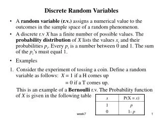
Discrete Random Variables. Discrete Probability Distributions Binomial Distribution Poisson Distribution Hypergeometric Distribution. Discrete Probability Distributions. Discrete Random Variables – Sample Space includes all mutually exclusive outcomes

Discrete Random Variables
E N D
Presentation Transcript
Discrete Random Variables • Discrete Probability Distributions • Binomial Distribution • Poisson Distribution • Hypergeometric Distribution Econ10/Mgt 10 Stuffler
Discrete Probability Distributions Discrete Random Variables – Sample Space includes all mutually exclusive outcomes Probabilities – from subjective, frequency or subjective methods Two conditions apply: Econ10/Mgt 10 Stuffler
Discrete Probability Distributions Probability distributions can be estimated from relative frequencies. Consider the discrete (countable) number of televisions per household (millions) from US survey data: Econ10/Mgt 10 Stuffler
Discrete Probability Distributions Probability distributions can be estimated from relative frequencies. Consider the discrete (countable) number of televisions per household from US survey data: 1,218 ÷ 101,501 = 0.012 Econ10/Mgt 10 Stuffler
Discrete Probability Distributions Probability distributions can be estimated from relative frequencies. Consider the discrete (countable) number of televisions per household from US survey data: EX: P(X=4) = P(4) = 0.076 = 7.6% Econ10/Mgt 10 Stuffler
Discrete Probability Distributions What is the probability there is at least one television but no more than three in any given household? Econ10/Mgt 10 Stuffler
Discrete Probability Distributions What is the probability there is at least one television but no more than three in any given household? Econ10/Mgt 10 Stuffler
Discrete Probability Distributions What is the probability there is at least one television but no more than three in any given household? “at least one television but no more than three” P(1 ≤ X ≤ 3) = P(1) + P(2) + P(3) = .319 + .374 + .191 = .884 Econ10/Mgt 10 Stuffler
Discrete Probability Distributions Assume a mutual fund salesman knows that there is 20% chance of closing a sale on each call he makes. Econ10/Mgt 10 Stuffler
Discrete Probability Distributions What is the probability distribution of the number of sales if he plans to call three customers? Let S denote success, making a sale: P(S) = .20, then Sʹ, not making a sale: P(Sʹ) = .80 Econ10/Mgt 10 Stuffler
P(S)=.2 P(S’)=.8 Discrete Probability Distributions • Developing a Probability Distribution Tree Sales Call 1 Econ10/Mgt 10 Stuffler
P(S)=.2 P(S)=.2 P(S’)=.8 P(S)=.2 P(S’)=.8 P(S’)=.8 Discrete Probability Distributions • Developing a Probability Distribution Tree Sales Call 1 Sales Call 2 Econ10/Mgt 10 Stuffler
P(S)=.2 P(S)=.2 P(S’)=.8 P(S)=.2 P(S)=.2 P(S’)=.8 P(S’)=.8 P(S)=.2 P(S)=.2 P(S’)=.8 P(S’)=.8 P(S)=.2 P(S’)=.8 P(S’)=.8 Discrete Probability Distributions • Developing a Probability Distribution Tree Sales Call 1 Sales Call 2 Sales Call 3 S S S S S S’ S S’S S S’S’ S’S S S’S S’ S’S’S S’S’S’ Econ10/Mgt 10 Stuffler
P(S)=.2 P(S)=.2 P(S’)=.8 P(S)=.2 P(S)=.2 P(S’)=.8 P(S’)=.8 P(S)=.2 P(S)=.2 P(S’)=.8 P(S’)=.8 P(S)=.2 P(S’)=.8 P(S’)=.8 Discrete Probability Distributions • Developing a Probability Distribution Tree Sales Call 1 Sales Call 2 Sales Call 3 S S S S S S’ S S’S S S’S’ S’S S S’S S’ S’S’S S’S’S’ Econ10/Mgt 10 Stuffler
P(S)=.2 P(S)=.2 P(S’)=.8 P(S)=.2 P(S)=.2 ‘)=.8 P(S’)=.8 P(S)=.2 P(S)=.2 P(S’)=.8 P(S’)=.8 P(S)=.2 P(S’)=.8 P(S’)=.8 Discrete Probability Distributions • Developing a Probability Distribution Sales Call 1 Sales Call 2 Sales Call 3 S S S S S S’ S S’S S S’S’ S’S S S’S S’ S’S’S S’S’S’ • X P(x) • .23 = .008 • 3(.032)=.096 • 3(.128)=.384 • 0 .83 = .512 Econ10/Mgt 10 Stuffler
P(S)=.2 P(S)=.2 P(SC)=.8 P(S)=.2 P(S)=.2 P(SC)=.8 P(SC)=.8 P(S)=.2 P(S)=.2 P(SC)=.8 P(SC)=.8 P(S)=.2 P(SC)=.8 P(SC)=.8 Discrete Probability Distributions • Explain how to derive .032 and .128 Sales Call 1 Sales Call 2 Sales Call 3 S S S S S SC S SC S S SC SC SC S S SC S SC SC SC S SC SC SC • X P(x) • .23 = .008 • 3(.032)=.096 • 3(.128)=.384 • 0 .83 = .512 Econ10/Mgt 10 Stuffler
P(S)=.2 P(S)=.2 P(SC)=.8 P(S)=.2 P(S)=.2 P(SC)=.8 P(SC)=.8 P(S)=.2 P(S)=.2 P(SC)=.8 P(SC)=.8 P(S)=.2 P(SC)=.8 P(SC)=.8 Discrete Probability Distributions • The P(X=2) is: Sales Call 1 Sales Call 2 Sales Call 3 (.2)(.2)(.8)= .032 S S S S S SC S SC S S SC SC SC S S SC S SC SC SC S SC SC SC • X P(x) • .23 = .008 • 3(.032)=.096 • 3(.128)=.384 • 0 .83 = .512 Econ10/Mgt 10 Stuffler
Discrete Probability Distributions • A discrete probability distribution represents a population Example: Population of number of TVs per household Example: Population of sales call outcomes • Since we have populations, we can describe • them by computing various parameters: • Population Mean and Population Variance Econ10/Mgt 10 Stuffler
Discrete Probability Distributions • Population Mean (Expected Value) • - Weighted average of all values with the weights • being the probabilities • - Expected value of X, E(X) Econ10/Mgt 10 Stuffler
Discrete Probability Distributions Population variance - weighted average of the squared deviations from the mean. “Short cut” formula for the variance Standard deviation formula Econ10/Mgt 10 Stuffler
Discrete Probability Distributions Find the mean, variance, and standard deviation for the population of the number of color televisions per household. = 0(.012) + 1(.319) + 2(.374) + 3(.191) + 4(.076) + 5(.028) = 2.084 Econ10/Mgt 10 Stuffler
Discrete Probability Distributions Find the mean, variance, and standard deviation for the population of the number of color televisions per household. = (0 – 2.084)2(.012) + (1 – 2.084)2(.319)+…+(5 – 2.084)2(.028) = 1.107 Econ10/Mgt 10 Stuffler
Discrete Probability Distributions Find the mean, variance, and standard deviation for the population of the number of color televisions per household. = 1.052 Econ10/Mgt 10 Stuffler
Discrete Probability Distributions Special application of Expected Value Suppose the probability that an insurance agent makes a sale is .20 and after costs earns a commission of $525. If he/she does not make a sale, they must pay $75 in costs. What is their expected value from a sales call? Does the benefit exceed the cost or is the opposite true? Econ10/Mgt 10 Stuffler
Discrete Probability Distributions Special application of Expected Value Let X be the discrete random variable of making a sale call x P(x) x•P(x) Sale $ 525 .20 $ 105 No Sale - $ 75 .80 - $ 60 E(x) = μ = ∑ xP(x) = $ 45 Econ10/Mgt 10 Stuffler
Binomial Distribution • Binomial distribution is the probability distribution that results from doing a “binomial experiment” which have the properties: • Fixed number of identical trials, represented as n. • Each trial has two possible outcomes: a “success” or “failure” • For all trials, the probability of success, P(success)=p, and the probability of failure, P(failure)=1–p=q, are constant. • The trials are independent Econ10/Mgt 10 Stuffler
Several Binomial Distributions Econ10/Mgt 10 Stuffler
Binomial Distribution • Success and failure: labels for binomial experiment outcomes, no value judgment is implied. • EX: Coin flip results in either heads or tails. • If we define “heads” as success, then • “tails” is considered a failure. • Other binomial examples: • An election candidate wins or loses • An employee is male or female • A worker is employed or unemployed Econ10/Mgt 10 Stuffler
Binomial Distribution Binomial Formula: where x = number of successes in n trials, n – x = number of failures in n trials, px = the probability of success raised to the number of successes, and qn-x = probability of failure raised to the number of failures Econ10/Mgt 10 Stuffler
Binomial Distribution • The random variable of a binomial experiment is defined as the number of successes in the n trials, and is called the binomial random variable. • EX: Flip a fair coin 10 times • 1) Fixed number of trials n=10 • 2) Each trial has two possible outcomes {heads (success), • tails (failure)} • 3) P(success)= 0.50; P(failure)=1–0.50 = 0.50 • 4) The trials are independent (i.e. the outcome of heads on the • first flip will have no impact on subsequent coin flips). • Flipping a coin ten times is a binomial • experiment since all conditions are met. Econ10/Mgt 10 Stuffler
Binomial Distribution Another sales call example: Assume a mutual fund salesman knows that there is • 20% chance of closing a sale on each call he makes. We want to determine the probability of making two sales in three calls: P(sale) = .2 P(no sale) = .8 P(X=2) = 3! = .096 2!(3-2)! .22.8.8 Econ10/Mgt 10 Stuffler
Binomial Distribution Another sales call example: Assume a mutual fund salesman knows that there is 20% chance of closing a sale on each call he makes We want probability of making two sales in three calls P(sale) = .2 P(no sale) = .8 GOOD NEWS! Megastat→Probability→Discrete Distributions→Binomial Econ10/Mgt 10 Stuffler
Binomial Distribution Econ10/Mgt 10 Stuffler
Pat Statsly • Pat Statsly is a student (not a good student) taking a • statistics course. Pat’s exam strategy is to rely on luck • for the first test. The test consists of 10 multiple-choice • questions. Each question has five possible answers, only • one of which is correct. Pat plans to guess the answer • to each question. • What is the probability that Pat gets no answers correct? • What is the probability that Pat gets two answers correct? Econ10/Mgt 10 Stuffler
Pat Statsly n=10 P(correct) = p = 1/5 = .20 P(wrong) = q = .80 Is this a binomial experiment? Check the conditions Econ10/Mgt 10 Stuffler
Pat Statsly n=10 P(correct) = p = 1/5 = .20 P(wrong) = q = .80 Is this a binomial experiment?Check the conditions: There is a fixed finite number of trials (n=10). An answer can be either correct or incorrect. The probability of a correct answer (P(success)=.20) does not change from question to question. Each answer is independent of the others. Econ10/Mgt 10 Stuffler
Pat Statsly • n=10, and P(success) = .20 • What is the probability that Pat gets no answers correct? • EX: P(x=0) What’s the interpretation of this result? Econ10/Mgt 10 Stuffler
Pat Statsly • n=10, and P(success) = .20 • What is the probability that Pat gets no answers correct? • EX: P(x=0) Pat has about an 11% chance of getting no answers correct using the guessing strategy. Econ10/Mgt 10 Stuffler
Pat Statsly Econ10/Mgt 10 Stuffler
Pat Statsly • n=10, and P(success) = .20 • What is the probability that Pat gets two answers correct? • EX: P(x=2) Econ10/Mgt 10 Stuffler
Pat Statsly • We have been using the binomial probability distribution to find probabilities for individual values of x. • To answer the question: • “Find the probability that Pat fails the quiz” • requires a cumulative probability, that is, P(X ≤ x) • If a grade on the quiz is less than 50% (i.e. 5 questions • out of 10), that’s considered a failed quiz. Econ10/Mgt 10 Stuffler
Pat Statsly • We have been using the binomial probability distribution to find probabilities for individual values of x. • To answer the question: • “Find the probability that Pat fails the test” • requires a cumulative probability, that is, P(X ≤ x) • If a grade on the test is less than 50% (i.e., 5 questions • out of 10), that’s considered a failed test. • We want to know what is: P(X ≤ 4) to answer Econ10/Mgt 10 Stuffler
Pat Statsly P(X ≤ 4) = P(0) + P(1) + P(2) + P(3) + P(4) = .9672 What is the interpretation of this result? Econ10/Mgt 10 Stuffler
Pat Statsly Its about 97% probable that Pat will fail the test using the luck strategy and guessing at answers. Econ10/Mgt 10 Stuffler
Binomial Table • Calculating binomial probabilities by hand is tedious and • error prone. There is an easier way. Refer to Table E-6 in • the Appendices. For the Pat Statsly example,n=10, so go to • the n=10 table: • Look in the Column, p=.20 and substitute into: • P(X ≤ 4) = P(0) + P(1) + P(2) + P(3) + P(4) • P(X ≤ 4) = .1074 + .2684 + .3020 + .2013 + .0881 = .9672 • The probability of Pat failing the test is 96.72% Econ10/Mgt 10 Stuffler
Poisson Distribution • Named for Simeon Poisson, Poisson distribution - • Discrete probability distribution • There there are no trials • Number of independent events (successes) occurring in a fixed time period or region of space that occur with a known average rate such as, arrivals, departures, or accidents, number of baskets in a quarter, etc. Econ10/Mgt 10 Stuffler
Poisson Distribution • For example: • The number of cars arriving at a service station in 1 hour. (The interval of time is 1 hour.) • The number of flaws in a bolt of cloth. (The specific region is a bolt of cloth.) • The number of accidents in 1 day on a particular stretch of highway. (The interval is defined by both time, 1 day, and space, the particular stretch of highway.) Econ10/Mgt 10 Stuffler
Poisson Distribution • Poisson random variable - number of successes that occur in a period of time or an interval of space • EX: On average, 96 trucks arrive at a border crossing • every hour. • EX: Number of typographical errors in a new textbook • edition averages 1.5 per 100 pages. Econ10/Mgt 10 Stuffler
Poisson Distribution… • The Poisson random variable is the number of successes that occur in a period of time or an interval of space in a Poisson experiment. • EX: On average, 96 trucks arrive at a border crossing • every hour. • E.g. The number of typographic errors in a new textbook edition averages 1.5 per 100 pages. successes time period successes (?!) interval Econ10/Mgt 10 Stuffler
Poisson Distribution Poisson experiment has four defining characteristics or properties: The number of successes that occur in any interval is independent of the number of successes that occur in any other interval The probability of a success in an interval is the same for all equal-size intervals The probability of a success is proportional to the size of the interval Only one value is required to determine the probability of a designated number of events occurring during an interval Econ10/Mgt 10 Stuffler

