Download
1 / 57
570 likes | 600 Views
Explore the complexities of oceanic circulation through observations, theoretical models, and numerical simulations, focusing on the vertical coordinate system in ocean modeling. Learn about errors, mixing phenomena, and calibration techniques for advanced numerical tools. Delve into the key advantages and limitations of z-models, sigma-models, and isopycnic models.

E N D
Ocean Modeling in Quasi-Lagrangian Vertical Coordinates Eric Chassignet University of Miami/RSMAS
Our understanding of the oceanic circulation increases via observations, theory, analytical and numerical models, and laboratory experiments. • Ocean numerical models are now so sophisticated that the generated outputs can be as difficult to interpret as observations. • One of the main question is the quantification of the truncation errors introduced by the discretization of the Navier-Stokes equations. • In many cases, numerically induced mixing can be larger than observed. • Need for calibration of the tool, i.e., the numerical model
Outline • Choice of vertical coordinate • Lagrangian coordinates • Hybrid (or generalized) coordinates • Choice of the reference pressure and importance of thermobaricity • Overflow representation • Model evaluation • Concluding remarks
Rotating and stratified fluids=>dominance of lateral over vertical transport • Hence, it is traditional in ocean modeling to orient the two horizontal coordinates orthogonal to the local vertical direction as determined by gravity • The choice of the vertical coordinate system is the single most important aspect of an ocean model's design (DYNAMO, DAMÉE-NAB) and introduces the largest source of truncation error (for a given horizontal resolution) • The practical issues of representation and parameterization are often directly linked to the vertical coordinate choice(Griffies et al., 2000).
Considerations in Choosing a Vertical Coordinate • The vertical coordinate must be monotonic with depth for any stably stratified density profile • Changes in density due to numerics should be much smaller than changes due to physical processes • Coordinate surfaces should coincide with locally-referenced neutral surfaces to permit a nearly two-dimensional representation of advection and isoneutral mixing. • Thermobaric effects (i.e., compressibility dependence on T and S) should be included in the pressure gradient term
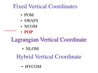
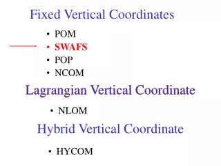
Currently, there arethree main vertical coordinates in use, none of which provides universal utility. “Development in Ocean Climate Modeling” by Griffies, Boening, Bryan, Chassignet, Gerdes, Hasumi, Hirst, Treguier, and Webb (2000, Ocean Modelling)
Key advantages of z-models • The simplest numerical discretization: this has allowed z-models to be used widely soon after their initial development • The equation of state for ocean water and the pressure gradient can be accurately represented • The surface mixed layer is naturally parameterized using z-coordinates
Disadvantages of z-models • The representation of tracer advection and diffusion along inclined density or neutral surfaces in the ocean interior is difficult (spurious numerically induced diapycnal mixing that can be much larger than the observed background values; see Griffies et al. 1998 for details) • Representation of bottom topography and parameterization of the bottom boundary layer is unnatural
Bottom boundary layer representation in z-coordinates From Beckmann and Doscher (1997)
Key advantages of sigma- (or terrain following) models • Smooth representation of the ocean bottom topography, with coordinate isolines concentrated in regions where bottom boundary layer processes are most important • Natural framework to parameterize bottom boundary layer processes.
Disadvantages of sigma-models • The surface mixed layer is not as well as with the z-coordinate. The vertical distance between grid points generally increases upon moving away from the continental shelf regions less vertical resolution • The horizontal pressure force consists of two sizable terms, each having separate numerical errors which generally do not cancel spurious pressure forces that drive nontrivial unphysical currents
Key advantages of isopycnic models • Tracer transport in the ocean interior occurs along directions defined by locally referenced potential density (i.e., neutral directions) no spurious numerical mixing as long as isopycnals are parallel to neutral directions • The bottom topography is represented in a piecewise linear fashion, hence avoiding the need to distinguish bottom from side as done with z-models
Disadvantages of isopycnic models • A density-coordinate is an inappropriate framework for representing the surface mixed layer or bottom boundary layer, since these boundary layers are mostly unstratified • Inclusion of thermobaricity in order to represent the effects of a realistic (nonlinear) equation of state is non-trivial
Outline • Choice of vertical coordinate • Lagrangian vertical coordinates • Hybrid (or generalized) coordinates • Choice of the reference pressure and importance of thermobaricity • Overflow representation • Model evaluation • Concluding remarks
Main design elements of a Lagrangian vertical coordinate • Depth (i.e., location of the vertical coordinate) is treated asdependentvariable. • One then needs to define a newindependentvariable “s ” capable of representing the 3rd (vertical) model dimension • Popular example: s = potential density
Continuity equation in generalized (“s”) coordinates (zero in fixedgrids) (zero in material coord.) (known)
Main design element of isopycnal models: Depthand (potential)densitytrade places asdependent / independentvariables - same number of unknowns, same number of (prognostic) equations, but different numerical properties Driving force for isopycnal model development:control of numerically induced diapycnal mixing and genetic diversity
Main benefits: - explicit PV and potential enstrophy conservation - reduction of numerically induced diapycnal mixing during advection & diffusion Main pitfalls: - degeneracy in unstratified water column - 2-term horizontal PGF is error-prone in steeply inclined layers (reduction to 1 term possible at the price of approximating equation of state) - layer outcropping (=> "massless" layers)
Outline • Choice of vertical coordinate • Lagrangian vertical coordinates • Hybrid (or generalized) coordinates • Choice of the reference pressure and importance of thermobaricity • Overflow representation • Model evaluation • Concluding remarks
Grid degeneracy is main reason for introducing hybrid vertical coordinate "Hybrid" means different things to different people: - linear combination of 2 or more conventional coordinates (examples: z+sigma, z+rho, z+rho+sigma) - ALE (Arbitrary Lagrangian-Eulerian) coordinate or generalized coordinate
MICOM HYCOM
ALE: “Arbitrary Lagrangian-Eulerian” coordinate • Original concept (Hirt et al., 1974): maintain Lagrangian character of coordinate but “re-grid” intermittently to keep grid points from fusing. • In HYCOM (HYbrid Coordinate Ocean Model), ALE is applied in the vertical only (1) to maintain minimum layer thickness; (2) to nudge an entropy-related thermo- dynamic variable toward a prescribed layer-specific “target” value by importing water from above or below. • Process (2) renders the grid quasi-isentropic
The prototype HYCOM “re-gridder” or “grid generator” (Bleck, 2002) Design Principles: • T/S conservative • Monotonicity-preserving (no new T/S extrema during re-gridding) • Layer too dense => entrain lighter water from above • Layer too light => entrain denser water from below • Maintain finite layer thickness in upper ocean but allow massless layers on sea floor • Minimize seasonal vertical migration of coordinate layers by keeping non-isopycnic layers near top of water column.
Ideally, an ocean general circulation model (OGCM) should • retain its water mass characteristics for centuries • (a characteristic of isopycnic coordinates), • (b) have high vertical resolution in the surface mixed layer (a characteristic of z-level coordinates) for a proper representation of thermodynamical and biochemical processes, • (c) maintain sufficient vertical resolution in unstratified • or weakly-stratified regions of the ocean, • (d) have high vertical resolution in coastal regions • (a characteristic of terrain-following coordinates).
HYCOM The hybrid coordinate is one that is isopycnalin the open, stratified ocean, but smoothly reverts to a terrain-following coordinate in shallow coastal regions, and to pressure coordinate in the mixed layer and/or unstratified seas. Flor ida Cuba
σ-z z σ Hybrid
1/25° HYCOM East Asian Seas Model Nested inside 1/6° HYCOM Pacific Basin Model Boundary conditions via one-way nesting and 6 hrly ECMWF 10 m atmospheric forcing
1/25° East Asian Seas HYCOM (nested inside 1/6° Pacific HYCOM) North-south velocity cross-section along 124.5°E, upper 400 m blue=westward flow red=eastward flow density front associated with sharp topographic feature (cannot be resolved with fixed coordinates) Isopycnals over shelf region Yellow Sea flow reversal with depth Snapshot on14 October East China Sea Yellow Sea z-levels and sigma-levels over shelf and in mixed layer Snapshot on12 April
Outline • Choice of vertical coordinate • Lagrangian vertical coordinates • Hybrid (or generalized) coordinates • Choice of the reference pressure and importance of thermobaricity • Overflow representation • Model evaluation • Concluding remarks
HYCOM North Atlantic 1º experiments(Chassignet et al., 2003) • The main difference between the and 2 experiments is due to the model's representation of AABW since there is no distinct water mass representing AABW in the discretization. • The differences between the 2 and *2 experiments illustrate the importance of thermobaricity. Without inclusion of the thermobaric effects, the pressure gradient above and below 2000 m does not take into account the modulation of seawater compressibility by potential temperature anomalies. Both the surface and deep circulation are much stronger in the experiment without thermobaricity. It is also only in the *2 experiment that the AABW can be seen flowing north along the eastern side of the domain.
SEA SURFACE HEIGHT • Sea Surface Height along 65o W • Weaker SSH gradient across Gulf Stream in EXP-HP than in the hybrid and isopycnic experiments • Strongest SSH gradient across Gulf Stream in EXP-H2 • SSH gradient of EXP-H*2 similar to that of the experiments
DEEP WATER TRANSPORT Streamfunction for > 27.8 (int=1 Sv)
Outline • Choice of vertical coordinate • Lagrangian vertical coordinates • Hybrid (or generalized) coordinates • Choice of the reference pressure and importance of thermobaricity • Overflow representation • Model evaluation • Concluding remarks
Overflow Representation • Strongly dependent on the choice of the vertical coordinate • In fixed coordinate models (z and σ), the numerically induced entrainment (i.e. mixing) is larger than observed => no need for parameterization, the focus is on reducing the mixing to below observations • In density coordinate models, the densest fluid will sink to the bottom => need for an entrainment parameterization
Denmark Straits Overflow Along 31°W Colder fresher water forms over the shelf in the Nordic Seas and spills over the Denmark Strait Temperature and entrains more saline Irminger Sea water Salinity Results from 1/12° Atlantic HYCOM
Strong Ri dependence Small Ri dependence
Sensitivity to the entrainment parameterization of Turner (1986) Papadakis et al. (2003)
KPP vs. Turner (1986) • The K-Profile parameterization (Large et al., 1994) is widely used in ocean models • KPP is derived from observations while Turner (1986) is primarily derived from laboratory experiments • There are non-oceanic aspect aspects in Turner (1986), i.e. lack of rotation, … • KPP is however a broad representation of the processes and may not be very relevant to overflows
Modification of KPP (Xu, in preparation) Richardson # dependence of the slope angle (Turner, 1986; Özgökmen and Chassignet, 2002; Chang et al., 2004)
Original KPP Modified KPP
Outline • Choice of vertical coordinate • Lagrangian vertical coordinates • Hybrid (or generalized) coordinates • Choice of the reference pressure and importance of thermobaricity • Overflow representation • Model evaluation • Concluding remarks
U.S. GODAE: Global ocean prediction with the HYbrid Coordinate Ocean Model (HYCOM) (http://hycom.rsmas.miami.edu) • A broad partnership of institutions that will collaborate in developing and demonstrating the performance and application of eddy-resolving, real-time global and basin-scale ocean prediction systems using HYCOM • Community Effort:NRL, U. of Miami, Los Alamos, NOAA/NCEP, NOAA/AOML, NOAA/PMEL, PSI, FNMOC, NAVOCEANO, SHOM, LEGI, OPeNDAP, UNC, Rutgers, USF, Fugro-GEOS, Orbimage, Shell, ExxonMobil
Outline • Choice of vertical coordinate • Lagrangian vertical coordinates • Hybrid (or generalized) coordinates • Choice of the reference pressure and importance of thermobaricity • Overflow representation • Model evaluation • Concluding remarks