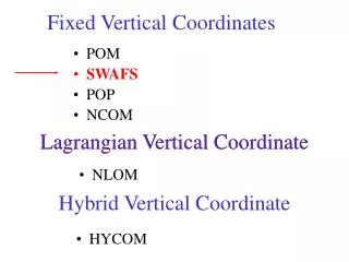
Fixed Vertical Coordinates
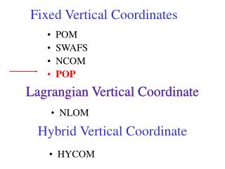
Fixed Vertical Coordinates. POM SWAFS NCOM POP. Lagrangian Vertical Coordinate. Lagrangian Vertical Coordinate. NLOM. Hybrid Vertical Coordinate. HYCOM. POP Parallel Ocean Program . Primary contacts: Mathew Maltrud, Rick Smith, & Phil Jones (LANL), Julie McClean (NPS)

Fixed Vertical Coordinates
E N D
Presentation Transcript
Fixed Vertical Coordinates • POM • SWAFS • NCOM • POP Lagrangian Vertical Coordinate Lagrangian Vertical Coordinate • NLOM Hybrid Vertical Coordinate • HYCOM
POPParallel Ocean Program Primary contacts: Mathew Maltrud, Rick Smith, & Phil Jones (LANL), Julie McClean (NPS) POP is based on the ocean code of Bryan (1969), Cox (1970;1984), and Semtner (1974). It was reconfigured for massively parallel computers (Smith et al., 1992) and can be run as ocean-only or coupled to air/ice/land components. It will likely be used as the ocean component of a high-resolution coupled synoptic prediction system at FNMOC. It will also be used for next-generation coupled climate prediction.
POPhttp://climate.acl.lanl.gov/models/pophttp://www.oc.nps.navy.mil/navypopPOPhttp://climate.acl.lanl.gov/models/pophttp://www.oc.nps.navy.mil/navypop Full-physics ocean general circulation model that includes packages to simulate mixed layer and other vertical and horizontal mixing processes. It is designed to run on multi-processor machines using domain decomposition in latitude and longitude. A user manual and the code is available from the LANL web site listed above. Some of the following material is taken from this manual.
Physics • Primitive equation • B-grid • Free-surface • Decoupled barotropic and baroclinic modes; solved using implicit and explicit schemes, respectively. • Several vertical mixing options are available • Several horizontal mixing options, for both momentum and tracers, are available • Variable depth (partial) bottom grid cells
Domain • POP is most commonly run in basin (North Atlantic) and global configurations. • The largest global POP domain run to date has 3600 x 2400 x 40 grid points. • The domain size can be constrained by architecture types.
North Atlantic POP domain. Note that the Gulf of Mexico is wrapped into Africa for computational efficiency. (Courtesy, J. McClean)
Grid and Coordinate System • POP can use a variety of grids as it allows any locally rectangular, orthogonal coordinate system on a sphere. • Vertical coordinate: z-level • Grids and topography are normally generated off-line; option to generate both horizontal and vertical grids and topography internally. • Grid Examples: • Mercator: Near-global and North Atlantic • Displaced North Pole global: North Pole is rotated into either North America, Asia, or Greenland, producing a smooth singularity-free grid in the Arctic ocean. This grid is matched to a Mercator grid in the Southern Hemisphere.
Spatial Resolution • The choice of resolution is determined by the problem to be understood, as well as available resources. • To date the highest horizontal resolution used for global POP is 0.1 (10 km at the equator decreasing to about 2-3 km in the Arctic). • 40 z-levels are being used for the global POP
Fully Global Displaced North Pole Grid Pole is rotated into Hudson Bay to avoid polar singularity. Average grid spacing is 12 km to 2.5 km Courtesy, McClean et al., 2001.
Boundary Conditions • “Sponge layers”: Graduated buffer zones at the boundaries of non-global models. They generate water mass properties from unresolved marginal seas. • PT and S are restored to climatological monthly PT and S. • Time scale is tapered from a maximum finite value at the boundary to 0 several degrees into the interior. • Closed boundaries (PT is potential temperature)
Forcing • Routines for specifying the surface forcing for the V, PT, and S, as well as interior forcing for PT and S are available. • Surface fluxes (wind stress, surface heat and freshwater flux) typically from ECMWF, NCEP or NOGAPS atmospheric prediction systems • For interior forcing, Levitus or MODAS climatologies are typically used • There are several options for how each type of forcing is applied: • How often: never, annual, monthly, hourly • Various methods for temporal interpolation to model time step
Initialization The user has the following options: • Climatological 3D PT and S • Restart from an earlier run • Create initial condition from a mean ocean profile of PT and S • Create initial condition from a 1992 Levitus mean ocean profile • The global model has been spun up over a 20-yr period with surface forcing
Data Assimilation • NRLMRY is running POP and Ocean MVOI together globally. • Other types of data assimilation schemes have been developed
Other Components • Coupling to NOGAPS underway (NRLMRY). • Will be coupled to LANL ice model (NPS and NRLMRY)
Implementation • Code: Fortran90 and MPI/Open MP • Runs in a Unix environment • Can be run on almost all computers (parallel and serial) • IBM SP3 @ NAVO: 44 global model days in 24 hours with 500 processors • Creation of grid, topography, forcing fields require separate Fortran codes
Output • Output is saved in the following formats • NetCDF • Binary (single precision) • Variables can be saved as • 2D snapshots at a chosen time interval e.g. daily SST • 3D snapshots at a chosen interval (history) e.g. 10-daily velocity fields • 3D averages over a specified period
References • Bryan, K., 1969: A numerical method for the study of the circulation of the world ocean. J. Comput. Phys., 4, 347-376. • Cox, M. D., 1970: A mathematical model of the Indian Ocean. Deep Sea Res., 17, 45-75. • Cox, M. D., 1984: A primitive equation three dimensional model of the ocean. GFDS Ocean Group Tech. Rep. 1, Geophys. Fluid Dyn. Lab./NOAA, Princeton Univ., Princeton, N. J., 250 pp. • Semtner, A. J., 1974: An oceanic general circulation model with bottom topography. Tech. Rep. 9, Dept. of Meteorol., Univ. of Calif., Los Angeles, 99 pp. • Smith, R. D., J. K. Dukowicz, and R. C. Malone, 1992: Parallel ocean circulation modeling. Physica D, 60, 38-61.
Fixed Vertical Coordinates • POM • SWAFS • NCOM • POP Lagrangian Vertical Coordinate Lagrangian Vertical Coordinate • NLOM Hybrid Vertical Coordinate • HYCOM
HYCOMHybrid Coordinate Ocean Model Primary contacts:E. Chassignet (U. Miami) / A. Wallcraft (NRL) HYCOM has evolved from the Miami Isopycnic Coordinate Ocean Model (MICOM), extending MICOM’s geographic range into coastal and unstratified seas. Sea ice and an advanced ocean data assimilation scheme will complete the high-resolution synoptic prediction system. It is planned to be transitioned to NAVO at a horizontal resolution of 0.08 in 2006 and at 0.04 by the end of the decade. It is also used in climate applications.
HYCOMhttp://hycom.rsmas.miami.edu Full-physics ocean general circulation model that includes packages to simulate mixed layer and other vertical and horizontal mixing processes. It is designed to run on multi-processor machines. Documentation and the source code are available at the web site. Some of the following material is taken from this manual.
Physics • Primitive equation, mass conserving • Free-surface • Flow and water properties along individual isopycnic layers are obtained using shallow water equations in each layer. Coordinates become nonisopycnic in shallow or unstratified seas when isopycnic layers collapse to zero at the bottom of the mixed layer. They transition to pressure-coordinates in the upper-ocean mixed layer (keep layer thicknesses constant in time) and standard terrain-following -coordinates in shallow water regions. • Includes full thermodynamics and complex equation of state • Several mixed layer options
Domain • It has been run at high-resolution (1/12 or higher) using basin (North Atlantic and North Pacific) and regional (Sea of Japan, Caribbean Sea, …) domains. • It has been run globally at lower resolution (1 and less) for climate applications.
Grid and Coordinate System • Hybrid vertical coordinate • Isopycnic in open, stratified ocean • Z-level in mixed layer and/or stratified seas • Terrain-following in shallow, coastal seas. • Horizontal coordinate: C-grid, Mercator projection • Global HYCOM has a Mercator grid to 59N and is joined to a bipolar projection across the Arctic which has 2 poles over land. This is known as the “Pan-Am” grid.
Currently, there are three main vertical coordinates in use, none of which provides universal utility. Hence, many developers have been motivated to pursue research into hybrid approaches. Courtesy: Chassignet (U. of Miami)
HYCOM The hybrid coordinate is one that is isopycnal in the open, stratified ocean, but smoothly reverts to a terrain-following coordinate in shallow coastal regions, and to pressure coordinate in the mixed layer and/or unstratified seas. Shaded field: density. Thin solid lines; layer interfaces. Orange line: mixed-layer depth. Depth range: 500 m. Numbers along bottom indicate latitude. Tick marks at the top and bottom indicate horizontal mesh size. Courtesy: Chassignet (U. of Miami)
A Mercator mesh of resolution is used south of 60ºN. At this latitude, the Mercator projection smoothly transitions to a bipolar projection with poles over Canada and Siberia, but without grid singularity over the ocean area. HYCOM GLOBAL CONFIGURATION Courtesy: Chassignet (U. of Miami)
HYCOM GLOBAL CONFIGURATION Courtesy: Chassignet (U. of Miami)
Spatial Resolution • To date the highest horizontal resolution used for basin-scale and regional HYCOM is 1/12 (0.08- North Atlantic and Pacific) and 1/32 (Sea of Japan), respectively. • The choice of resolution is determined by the problem to be understood as well as available resources.
Boundary Conditions • Relaxation of PT, S and vertical coordinate pressure levels in sponge layers. • Open boundaries. • Closed boundaries.
Forcing • Surface forcing: climatological ECMWF and HR + 6-hourly NOGAPS • wind stress, wind speed • heat flux (using bulk formula), • evaporation - precipitation + relaxation to climatological SSS
Initialization The user has the following options • Climatological 3D PT and S • Restart from an earlier run.
Data Assimilation • Current (1/3 Atlantic version of HYCOM) • Assimilation of MODAS optimally-interpolated SSH anomalies from satellite altimetry • Vertical projection of the surface observations to depth • Running in real time • Research & Development • Various filter schemes are being investigated
Assimilation of MODAS SSH analyzed fields NO ASSIMILATION 1/3° Atlantic HYCOM SSH20 November 2000 Independent frontal analysis of IR observations performed at NAVO overlaid. White line shows the part of the front being observed within the last 4 days. Black line shows the part of the front older than 4 days. Courtesy: Smedstad
1/3° Atlantic HYCOM SSH30 July 2001 Independent frontal analysis of IR observations performed at NAVO overlaid. White line shows the part of the front being observed within the last 4 days. Black line shows the part of the front older than 4 days. Courtesy: Smedstad
Implementation • Code: Fortran90 and OpenMP/MPI • Runs in a Unix environment • Can be run on almost all computers (both serial and parallel). • Creation of grid, topography, forcing fields require separate Fortran codes
Output • Variables can be saved as • 2-D snapshots at a chosen time interval e.g. daily SST. These are movie files. • 3-D averages over a specified period
References • Peer Reviewed Publications • Thacker, W.C. and O. E. Esenkov: Assimilating XBT data into HYCOM, Journal of Atmospheric and Oceanic Technology, Vol. 19, No. 5, 709-724, 2002. • Bleck, R.: An Oceanic General Circulation Model Framed in Hybrid Isopycnic-Cartesian Coordinates, Ocean Modelling, Vol. 4, 55-88, 2002. • Stammer, D., and E.P. Chassignet, 2000: Ocean state estimation and prediction in support of oceanographic research. Oceanography, 13, 51-56. • Non Peer Reviewed Publications (see WEB site) • Bleck, R., Formulation of the horizontal pressure gradient force (PGF) in generalized coordinates (Posted March 14, 2001) • Bleck, R., Generalized Coordinate Treatment in HYCOM (Posted: November 27, 2000)