Download

1 / 16
190 likes | 534 Views
The Solow Growth Model (Part One). The steady state level of capital and how savings affects output and economic growth. Model Background.

E N D
The Solow Growth Model (Part One) The steady state level of capital and how savings affects output and economic growth.
Model Background • Previous models such as the closed economy and small open economy models provide a static view of the economy at a given point in time. The Solow growth model allows us a dynamic view of how savings affects the economy over time.
Building the Model: goods market supply • We begin with a production function and assume constant returns.Y=F(K,L) so… zY=F(zK,zL) • By setting z=1/L we create a per worker function.Y/L=F(K/L,1) • So, output per worker is a function of capital per worker. We write this as,y=f(k)
Building the Model: goods market supply y=f(k) y k • The slope of this function is the marginal product of capital per worker.MPK = f(k+1)–f(k) • It tells us the change in output per worker that results when we increase the capital per worker by one. Change in y Change in k
Building the Model:goods market demand • We begin with per worker consumption and investment. (Government purchases and net exports are not included in the Solow model). This gives us the following per worker national income accounting identity.y = c+I • Given a savings rate (s) and a consumption rate (1–s) we can generate a consumption function.c = (1–s)y …which makes our identity,y = (1–s)y + I …rearranging,i = s*y …so investment per worker equals savings per worker.
Steady State Equilibrium • The Solow model long run equilibrium occurs at the point where both (y) and (k) are constant. These are the endogenous variables in the model. • The exogenous variable is (s).
Steady State Equilibrium • By substituting f(k) for (y), the investment per worker function (i = s*y) becomes a function of capital per worker (i = s*f(k)). • To augment the model we define a depreciation rate (δ). • To see the impact of investment and depreciation on capital we develop the following (change in capital) formula,Δk = i – δk …substituting for (i) gives us,Δk = s*f(k) – δk
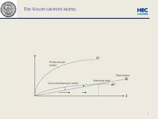
Steady State Equilibrium δk s*f(k),δk s*f(k) s*f(k*)=δk* k klow k* khigh • At the point where both (k) and (y) are constant it must be the case that, Δk = s*f(k) – δk = 0 …or, s*f(k) = δk…this occurs at our equilibrium point k*. • If our initial allocation of (k) were too high, (k) would decrease because depreciation exceedsinvestment. • If our initial allocation were too low, k would increase because investment exceeds depreciation. • At k* depreciation equals investment.
Steady State Equilibrium (getting there) δk s*f(k),δk s*f(k) s*f(k*)=δk* k k* • Suppose our initial allocation of (k1) were too low. k2=k1+Δk k3=k2+Δk k4=k3+Δk k5=k4+Δk … This process continues until we converge to k* k1 k2 k3 k4 k5 K2 is still too low so… K3 is still too low so… K4 is still too low so… K5 is still too low so…
A Numerical Example • Starting with the Cobb-Douglas production function we can arrive at our per worker production as follows,Y=K1/2L1/2…dividing by L,Y/L=(K/L)1/2…or,y=k1/2 • recall that (k) changes until,Δk=s*f(k)–δk=0 ...i.e. until, s*f(k)=δk
A Numerical Example • Given s, δ, and initial k, we can compute time paths for our variables as we approach the steady state. • Let’s assume s=.4, δ=.09, and k=4. • To solve for equilibrium set s*f(k)=δk. This gives us .4*k1/2=.09*k. Simplifying gives us k=19.7531, so k*=19.7531.
A Numerical Example • But what it the time path toward k*? To get this use the following algorithm for each period. • k=4, and y=k1/2 , so y=2. • c=(1–s)y, and s=.4, so c=.6y=1.2 • i=s*y, so i=.8 • δk =.09*4=.36 • Δk=s*y–δk so Δk=.8–.36=.44 • so k=4+.44=4.44 for the next period.
A Numerical Example • Repeating the process gives…
A Numerical Example • Graphing our results in Mathematica gives us,
Changing the exogenous variable - savings δk s*f(k),δk s*f(k) s*f(k*)=δk* k k* • We know that steady state is at the point where s*f(k)=δk s*f(k*)=δk* s*f(k) • What happens if we increase savings? • This would increase the slope of our investment function and cause the function to shift up. k** • This would lead to a higher steady state level of capital. • Similarly a lower savings rate leads to a lower steady state level of capital.
Conclusion • The Solow Growth model is a dynamic model that allows us to see how our endogenous variables capital per worker and output per worker are affected by the exogenous variable savings. We also see how parameters such as depreciation enter the model, and finally the effects that initial capital allocations have on the time paths toward equilibrium. • In the next section we augment this model to include changes in other exogenous variables; population and technological growth.