Download
1 / 24
260 likes | 323 Views
Chapter 5 – second lecture. Introducing Advanced Macroeconomics: Growth and business cycles. TECHNOLOGICAL PROGRESS AND GROWTH: THE GENERAL SOLOW MODEL. The complete Solow model. Analyzing the Solow model (see previous lecture). Define: and From we get

E N D
Chapter 5 – second lecture Introducing Advanced Macroeconomics: Growth and business cycles TECHNOLOGICAL PROGRESS AND GROWTH: THE GENERAL SOLOW MODEL
Analyzing the Solow model (see previous lecture) • Define: and • From we get • From and we get • Dividing by on both sides gives
Inserting gives the transition equation: • Subtracting from both sides gives the Solow equation: • Dividing by on both sides to get the modified Solow equation:
Previous lecture • Using the transition equation and the transition diagram we showed convergence to steady state: . • We derived some relevant steady state growth paths e.g.: • We showed that there is balanced growth in steady state with and growing at the same positive growth rate, , and with a constant real interest rate, . • We discussed structural policy aimed at affecting steady state. • We showed and discussed empirics for steady state:The model substantially underestimates the impact of the structural parameters on GDP per worker!
This lecture • Comparative analysis in the Solow diagrams. • The convergence process. • Growth accounting.
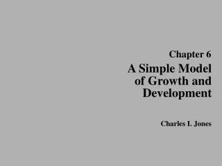
Comparative analysis in the Solow diagrams • Initially the economy is in steady state at parameters and . The savings rate increases permanently from to .
Old steady state: and , and and both grow at rate , the lower line below: • New steady state: and , and and grow at rate , but along a higher growth path, the upper line above.
Transition: grows from up to . The growth rate of jumps up and then gradually falls back to zero. From follows that . Hence, during the transition, grows at a larger rate than , and jumps up and then falls gradually back to . The growth rate of jumps too, since .
Convergence in the Solow model The modified Solow diagram again: There is accordance with conditional convergence: Two countries with the same …
The process of convergence empirically • What does the model tell us more precisely about the process of convergence , i.e., how does growth in each country depend on structural parameters and initial position? • Using the transition equation, we derive a formula for the growth rate of . To do this we linearize around steady state etc. • Differentiating wrt. and evaluating in steady state gives It’s easy to see that .
Mathematical note: consider a differentiable function, going through the point , so . Then: If furthermore, then: • Use (1) on in to find that • This is an approximation of the dynamics of the Solow model, and it’s a linear one! • The linear difference equation implies stability of , since .
Use again , this time on : • Use this to rewrite : • Use that from one has : • The convergence property: in each period, a constant fraction of the remaining gap is closed. The rate of convergence is
We now derive the solution to the difference equation: • The characteristic polynomial is and the associated root is . The complete solution to the homogeneous equation is: . • A specific solution to the non-homogeneous is: , implying that the complete solution is: • For the constant to fit with the initial situation: . • Hence the solution is:
Using the solution for etc. gives: • Inserting for and our expresssion for gives the convergence equation: • Rewrite slightly:
Assuming that and are the same in all countries, this suggests a regression equation: • OLS estimation across 90 countries over the period 1960-2000 gives: • Plotting against gives
Positive aspects: significant parameters, relatively high R2 etc. This does not crucially conflict with the assumption of the same and in all countries. But: • We have two estimates of the rate of convergence: • From theory: • From empirics: Together with an estimated of and this gives The model substantially overestimates the rate of convergence! • Confronted with empirics, the Solow model does quite well, both with respect to its steady state and its convergence prediction. However, in both cases there is an empirical problem of magnitudes. It could have been better, but it’s still a very well-performing model.
Growth accounting • With data for and (which often is availible) and with we can compute as a residual. We call this the Solow residual. • Why not growth accounting in levels?
Growth accounting per capita (worker) • With data for and and with we can once more compute the Solow residual, . • We can use this residual to check the underlying ”technological growth”
Conclusions, the general Solow model • Implications for economic policies are more or less the same as those derived from the basic Solow model. • The model implies convergence to a steady state with balanced growth and with a constant, positive growth rate of GDP per worker. Thus, the steady state prediction of the model is in accordance with a fundamental ”stylized fact”. However, the underlying source of growth, technological progress, is not explained. • The steady state prediction performs quite well empirically, but the model underestimates the effect of the savings rate and the growth rate of the labour force on income per worker. • The convergence prediction also performs well empirically, but the model overestimates the rate of convergence.