Download
1 / 18
190 likes | 246 Views
Explore the General Solow Model's insights on economic growth through technological advancements. Learn about steady states, balanced growth rates, and structural policies for prosperity in a closed economy. Dive into the analysis of convergence towards constant levels for capital and labor. Understand the implications of exogenous technological progress on GDP growth per worker.

E N D
Chapter 5 – first lecture Introducing Advanced Macroeconomics: Growth and business cycles TECHNOLOGICAL PROGRESS AND GROWTH: THE GENERAL SOLOW MODEL
The general Solow model • Back to a closed economy. • In the basic Solow model: no growth in GDP per worker in steady state. This contradicts the empirics for the Western world (stylized fact #5). In the general Solow model: • Total factor productivity, , is assumed to grow at a constant, exogenous rate (the only change). This implies a steady state with balanced growth and a constant, positive growth rate of GDP per worker. • The source of long run growth in GDP per worker in this model is exogenous technological growth. Not deep, but: • it’s not trivial that the result is balanced growth in steady state, • reassuring for applications that the model is in accordance with a fundamental empirical regularity. • Our focus is still: what creates economic progress and prosperity…
The micro world of the Solow model … is the same as in the basic Solow model, e.g.: • The same object (a closed economy). • The same goods and markets. Once again, markets are competitive with real prices of 1, and , respectively. There is one type of output (one sector model). • The same agents: consumers and firms (and government), essentially with the same behaviour, specifically: one representative profit maximising firm decides and given and . • One difference: the production function. There is a possibility of technological progress: The full sequence is exogenous and for all . Special case is (basic Solow model).
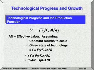
The production function with technological progress with a given sequence, with a given sequence, • With a Cobb-Douglas production function it makes no difference whether we describe technical progress by a sequence, , for TFP or by the corresponding sequence, , for labour augmenting productivity. • In our case the latter is the most convenient. The exogenous sequence, , is given by: • Technical progress comes as ”manna from heaven” (it requires no input of production).
Remember the definitions: and . • Dividing by on both sides of gives the per capita production function: • From this follows: Growth in can come from exactly two sources, and is the weighted average of and with weights and . • If, as in balanced growth, is constant, then !
The complete Solow model • Parameters: . Let . • State variables: and . • Full model? Yes, given and the model determines the full sequences
Note: That is: capital’s share , labour’s share , pure profits . Our should still be around . • Also note: defining ”effective labour input” as :The model is matematically equivalent to the basic Solow model with taking the place of , and taking the place of , and with !We could, in principle, take over the full analysis from the basic Solow model, but we will nevertheless be…
Analyzing the general Solow model • If the model implies convergence to a steady state with balanced growth, then in steady state and must grow at the same constant rate (recall again that is constant under balanced growth). Remember also: Hence if , then . If there is convergence towards a steady state with balanced growth, then in this steady state and will both grow at the same rate as and hence and will be constant. • Furthermore: from the above mentioned equivalence to the basic Solow model, and converge towards constant steady state values. • Each of the above observations suggests analyzing the model in terms of:
and • From we get • From and we get • Dividing by on both sides gives • Inserting gives the transition equation: • Subtracting from both sides gives the Solow equation:
Convergence to steady state:the transition diagram • The transition equation is: • It is everywhere increasing and passes through (0,0). • The slope of the transition curve at any is: • We observe: . Furthermore, . We assume that the latter very plausible stability condition is fulfilled.
Convergence of to the intersection point follows from the diagram. Correspondingly: . Some first conclusions are: • In the long run, and converge to constant levels, and , respectively. These levels define steady state. • In steady state, and both grow at the same rate as , that is, at the rate and the capital output ratio, , must be constant.
Steady state • The Solow equationtogether with gives: • Using and we get the steady state growth paths:
Since , • It also easily follows from that • There is balanced growth in steady state: and grow at the same constant rate, , and is constant. • There is positive growth in GDP per capita in steady state (provided that ).
Structural policies for steady state • Output per capita and consumption per capita in steady state are: • Golden rule: the , that maximises the entire path, . Again: . • The elasticities of wrt. and are again and , respectively. • Policy implications from steady state are as in the basic Solow model: encourage savings and control population growth. • But we have a new parameter, ( corresponds to ). We want a large , but it is not easy to derive policy conclusions wrt. technology enhancement from our model ( is exogenous).
Empirics for steady state • Assume that all countries are in steady state in 2000! • It’s hard to get good data for , so make the heroic assumption that is the same for all countries in 2000. • Set (plausibly) • If is GDP per worker in 2000 of country , the above equation suggests the following regression equation:with and measured appropriately (here as averages over 1960-2000), and where
High significance! Large R2! Even though we have assumed that is the same in all countries! • But always remember the problem of correlation vs. causality. • Furthermore: the estimated value of is not in accordance with the theoretical (model-predicted) value of . Or: • The conclusion is mixed: the figure on the previous slide is impressive, but the figure’s line is much steeper than the model suggests.