Download
1 / 14
310 likes | 931 Views
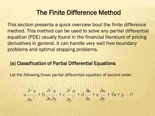
Chapter 6 Basics of Finite Difference. OUTLINE 6.1 Components of Numerical Methods 6.2 Introduction to Finite Difference 6-3 Errors Involved in Numerical Solutions 6-4 Example. 6.1 Components of numerical methods (3) Discretization methods (Finite Difference)-1.

E N D
Chapter 6 Basics of Finite Difference OUTLINE 6.1 Components of Numerical Methods 6.2 Introduction to Finite Difference 6-3 Errors Involved in Numerical Solutions 6-4 Example
6.1 Components of numerical methods (3) Discretization methods (Finite Difference)-1 • First step in obtaining a numerical solution is to discretize the geometric domain to define a numerical grid • Each node has one unknown and need one algebraic equation, which is a relation between the variable value at that node and those at some of the neighboring nodes. • The approach is to replace each term of the PDE at the particular node by a finite-difference approximation. • Numbers of equations and unknowns must be equal 6-3
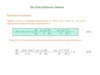
6.1 Components of numerical methods (4) Discretization methods (Finite Difference)-2 • Taylor Series Expansion: Any continuous differentiable function, in the vicinity of xi, can be expressed as a Taylor series: • Higher order derivatives are unknown and can be dropped when the distance between grid points is small. • By writing Taylor series at different nodes, xi-1, xi+1, or both xi-1 and xi+1, we can have: Forward-FDS Backward-FDS 1st order, order of accuracy Pkest=1 Central-FDS 2nd order, order of accuracy Pkest=1 6-4
6-2 Introduction to Finite Difference (1) • Numerical solutions can give answers at only discrete points in the domain, called grid points. • If the PDEs are totally replaced by a system of algebraic equations which can be solved for the values of the flow-field variables at the discrete points only, in this sense, the original PDEs have been discretized. Moreover, this method of discretization is called the method of finite differences. 6-5
6-2 Introduction to Finite Difference (2) • A partial derivative replaced with a suitable algebraic difference quotient is called finite difference. Most finite-difference representations of derivatives are based on Taylor’s series expansion. • Taylor’s series expansion: Consider a continuous function of x, namely, f(x), with all derivatives defined at x. Then, the value of f at a location can be estimated from a Taylor series expanded about point x, that is, • In general, to obtain more accuracy, additional higher-order terms must be included. 6-6
6-2 Introduction to Finite Difference (4) • Forward, Backward and Central Differences: (1) Forward difference: Neglecting higher-order terms, we can get (a) 6-8
6-2 Introduction to Finite Difference (5) (2) Backward difference: Neglecting higher-order terms, we can get (3) Central difference: (a)-(b) and neglecting higher-order terms, we can get (b) …(c) 6-9
6-2 Introduction to Finite Difference (6) (4) If , then (a), (b), (c) can be expressed as Forward: Backward: Central: Note: …(d) …(e) …(f) 6-10
6-2 Introduction to Finite Difference (7) • Truncation error: The higher-order term neglecting in Eqs. (a), (b), (c) constitute the truncation error. The general form of Eqs. (d), (e), (f) plus truncated terms can be written as Forward: Backward: Central: 6-11
6-2 Introduction to Finite Difference (8) • Second derivatives: * Central difference: If , then (a)+(b) becomes * Forward difference: * Backward difference: 6-12
6-2 Introduction to Finite Difference (9) • Mixed derivatives: * Taylor series expansion: * Central difference: * Forward difference: * Backward difference: 6-13
6-3 Errors Involved in Numerical Solutions (1) • In the solution of differential equations with finite differences, a variety of schemes are available for the discretization of derivatives and the solution of the resulting system of algebraic equations. • In many situations, questions arise regarding the round-off and truncation errors involved in the numerical computations, as well as the consistency, stability and the convergence of the finite difference scheme. • Round-off errors:computations are rarely made in exact arithmetic. This means that real numbers are represented in “floating point” form and as a result, errors are caused due to the rounding-off of the real numbers. In extreme cases such errors, called “round-off” errors, can accumulate and become a main source of error. 6-23
6-3 Errors Involved in Numerical Solutions (2) • Truncation error: In finite difference representation of derivative with Taylor’s series expansion, the higher order terms are neglected by truncating the series and the error caused as a result of such truncation is called the “truncation error”. • The truncation error identifies the difference between the exact solution of a differential equation and its finite difference solution without round-off error. 6-24