Finite Difference Methods

1. Finite Difference Methods 18-20 September 2012

2. Thematic Outline • Methods for computing temporal finite differences • Methods for computing spatial finite differences • Applications of grid staggering • Impacts of truncation error that arises from the finite difference approximations

3. Temporal Finite Differences • Note: the temporal differencing methods to be discussed apply to grid-point and spectral models. • Two types of time differencing schemes… • Explicit: all future time terms appear on one side of an equation • Implicit: future time terms appear on both sides of an equation • Hybrid explicit/implicit schemes also exist. • Explicit differences can be solved directly; implicit differences must be solved iteratively.

4. Explicit Temporal Differences • Two methods… • Single step (forward and centered differences) • Multiple step (predictor-corrector methods) • Single step example, centered difference: where f is some dependent field (u, v, T, etc.) and F is the forcing on that field

5. Explicit Temporal Differences • Single step example, forward-in-time difference: • Let us consider these in the context of a real-world example, a one-dimensional advection equation…

6. Explicit Temporal Differences • Centered difference: • Forward-in-time difference: Note: in both cases, we applied a second-order centered finite difference in space. We’ll discuss this method further shortly.

7. Explicit Temporal Differences • In predictor-corrector schemes, a prediction for the dependent field at some future time is first made using some finite difference approximation. • From this, the forcing at that future time is obtained, whether from finite difference or spectral methods. • That forcing is then used, often with a forward-in-time difference, to integrate to the next time.

8. Explicit Temporal Differences • Example: Runge-Kutta type scheme… • Predict: • With f*, obtain F*. • Predict: • With fτ, obtain Fτ. • Correct: • Predictor-corrector methods provide superior accuracy at the expense of efficiency.

9. Explicit Temporal Differences • Issue: acoustic and other fast-moving waves • These waves require small time steps to maintain computational stability in the advection terms (CFL) • If not filtered, how to handle need for a small time step? • Potential method: split-explicit schemes • Small ∆t for terms representing fast-moving waves • Large ∆t for terms representing slower-moving waves • Reduces number of computations on short time steps • Commonly used with current mesoscale model systems

10. Implicit Temporal Differences • In explicit schemes, the forcing terms (spatial derivatives) are evaluated only at the initial time t. • In implicit schemes, these terms are evaluated at the future time t+1 and the initial time t. • In other words, they are valid at t+1/2. • Thus, terms at t+1 appear on both sides of the equation and the time derivative must be solved iteratively.

11. Implicit Temporal Differences • Let us again consider the example of a one-dimensional advection equation… • Explicit, forward-in-time approximation: • Instead of representing the spatial derivative exclusively at t=t, let us represent it as the average of its values at the initial (t) and future (t+1) times…

12. Implicit Temporal Differences • Spatial finite difference approximation: • If we substitute and apply a second-order centered spatial finite difference, this gives us equation (3.21),

13. Implicit Temporal Differences • Advantage: implicit schemes are typically unconditionally stable • CFL criterion for advection terms is thus not a concern • Enables us to use a longer time step to handle all waves • Disadvantage: iterative nature requires more computations per time step than explicit schemes Longer time step savings < iterative computational expense

14. Implicit Temporal Differences • To alleviate these issues, semi-implicit methods may be used. • Meteorological terms: handled explicitly • Non-meteorological terms: handled implicitly • Alleviating the need for a small time step to maintain linear stability that arises with explicit methods. • A common, long time step may be used for all terms because implicit terms are stable for all time steps. • Advantage over split-explicit schemes. • Iterative computational expense is still present, however.

15. Spatial Differencing • We must first establish our frame of reference: fixed to the Earth or fixed to air parcels. • Thus far, we have considered a frame of reference tied to the Earth, an Eulerian reference frame. • All terms are defined and computed on a fixed grid. • Example: 1-D advection equation… ∆x ∆x x-1 x x+1

16. Spatial Differencing • But, as we’ve discussed before, the CFL criterion applies to the advection terms in this framework. • Can we utilize a reference frame that encompasses the advection terms and eliminates this issue? • Yes – if we use a reference frame tied to the motion (i.e., fixed to air parcels)!

17. Spatial Differencing • Such a reference frame is known as a Lagrangian reference frame. • Because Lagrangian methods follow air parcels, the spatial and vertical resolutions of the model are flow-dependent. • Finer resolution is found in convergent regions. • Coarser resolution is found in divergent regions. • This is not ideal.

18. Spatial Differencing • Alternative: semi-Lagrangian methods • In a Lagrangian framework, only one set of parcels is followed, but is followed over all time steps. • In a semi-Lagrangian framework, a new set of parcels (defined by the chosen grid) is followed at each time step. • Parcels are followed utilizing parcel trajectories. • Either forward or backward trajectories may be used. • The spatial derivatives (advection terms) are implicitly accounted for by the along-trajectory evolution.

19. Semi-Lagrangian Differencing • Example: forward trajectories • Evenly-spaced grid (black) is defined at t=t. • Trajectories (red lines) are released from each grid point and followed forward in time to t=t+1 (red dots). • Non-advection terms in the primitive equations change the values of atmospheric fields along the trajectories. • The values of these fields at t=t+1 are then interpolated back to a uniform grid and the process repeated. x-1 x x+1

20. Semi-Lagrangian Differencing • Example: backward trajectories • Evenly-spaced grid (black) is defined at t=t+1. • Trajectories (red lines) are released from each grid point and followed backward in time to t=t (red dots). • Non-advection terms in the primitive equations change the values of atmospheric fields along the trajectories. • Need to interpolate from evenly-spaced grid valid at t=t to obtain this forcing. • But, no interpolation needed for t=t+1 – already on uniform grid! x-1 x x+1

21. Semi-Lagrangian Differencing • Backward trajectory methods are preferred. • Easier to interpolate from evenly-spaced grids to non-gridded trajectory locations than the inverse. • But, how can we represent the example on the previous slide numerically (and not just graphically)?

22. Semi-Lagrangian Differencing Imagine a two-dimensional grid, as below, at t=t+1. Our parcel location at this time is given by (i,j). (i,j)

23. Semi-Lagrangian Differencing The backward trajectory from (i,j) is given by the red line. The parcel locations at t=t-1 (x) and t=t (+) are noted in blue. X + (i,j)

24. Semi-Lagrangian Differencing Let the location of X be and the location of + be . X + (i,j)

25. Semi-Lagrangian Differencing • Let the dependent variable in question be given by f and the forcing by F. • We want ft+1 and know ft-1 and ft by interpolation between grid points at the previous times. • F is computed locally using Eulerian finite difference methods and then interpolated between grid points. • The finite difference can then be explicit or implicit.

26. Semi-Lagrangian Differencing • Explicit: recall our centered-in-time difference... • The values of ft+1, ft-1, and Ft are taken at their locations along the trajectory, i.e.,

27. Semi-Lagrangian Differencing • Implicit: a generic example can be expressed as... • As for the explicit case, the values of ft+1, ft, Ft+1, and Ft are taken at their locations along the trajectory,

28. Semi-Lagrangian Differencing • Advantages of semi-Lagrangian schemes... • Loss of advection terms eliminates CFL criterion, enabling the usage of a longer time step. • Can be used for either grid point or spectral methods. • Can also be used with semi-implicit differencing schemes. • Minimizes non-linear instability (to be discussed soon). • Disadvantage of semi-Lagrangian schemes… • Not energy or mass conserving (a particular problem over long model integrations)

29. Grid Staggering • For some applications, it can be useful to define our dependent variables on two slightly offset grids. • This is known as grid staggering. • Both horizontal and vertical grid staggering are possible. • A typical staggering increment is ½ the grid interval. • Which variables apply to each grid depends upon the desired computational characteristics.

30. Grid Staggering simple 1-D example for u and θ • (a): must use θj+1 and θj-1 (over 2∆x) to compute a centered finite difference • (b): can use θj+½ and θj-½ (over ∆x) to compute a centered finite difference • Staggering halves the effective grid increment and minimizes the impacts of truncation error on the solution.

31. Grid Staggering • There are many examples of staggered grids in current NWP models. • Arakawa C-grid: mass variables staggered from kinematic variables; used in WRF-ARW model

32. Grid Staggering • Other staggers… • Arakawa B-grid: akin to C grid, but with mass and kinematic variables staggered on grid centers and corners rather than grid centers and sides • Arakawa E-grid: akin to C grid, except rotated 45° • These grids are used by the MM5/NMM-B and WRF-NMM mesoscale models, respectively.

33. Grid Staggering • Grid staggering increases effective resolution but does not increase the number of grid points. • Increase in effective resolution requires a smaller time step to meet CFL criterion. • Only if Eulerian differencing methods are used, however. • Recall: as ∆x decreases, Courant number increases. • The benefit from reduced truncation error outweighs time step considerations, however.

34. Truncation Error • Many of the primitive equations are differential equations with partial derivative terms. • If we utilize grid point methods, these terms must be approximated with finite differences. • These approximations introduce error, however, depending upon their complexity. • This error is known as truncation error.

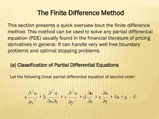
35. Finite Difference Approximations • First, however, it is useful to revisit how finite difference approximations are obtained. • Any function over an interval – i.e., a partial derivative – can be approximated by a Taylor series. • Generally, for a function in x,

36. Finite Difference Approximations • Expanded to several terms, we obtain (3.24), • Here, a is our point of interest and x is some point of reference. R is a residual term representing the error.

37. Finite Difference Approximations • This equation is used to obtain finite difference approximations for the function f. • The accuracy of each approximation is dependent upon the highest power/order terms retained in the equation. • Retain higher order terms: increased accuracy. • Keep only lower order terms: decreased accuracy.

38. Finite Difference Approximations • Example: first order / two point, forward in space • Let x = a+∆x and truncate 2nd order and higher terms… • Solve for the derivative…

39. Finite Difference Approximations • Example: first order / two point, backward in space • Let x = a-∆x and truncate 2nd order and higher terms… • Solve for the derivative… • First order schemes are typically not used, however, because they have large truncation errors.

40. Finite Difference Approximations • Example: second order / three point, centered • Let x = a+∆x and truncate 3nd order and higher terms… • Let x = a-∆x and truncate 3nd order and higher terms…

41. Finite Difference Approximations • Subtract the 2nd equation from the first… • Solve for the first derivative…

42. Finite Difference Approximations • A five point / 4th order approximation is given by… where the two closest points on each side of a are used in the calculation of the derivative. • Any of these – or even higher-order – expressions may be used in numerical models to compute spatial derivatives in physical / grid-point space.

43. Truncation Error • Example: let f be a function for which the derivative is exactly known and compare that result to the finite difference approximations. • As in the text, let f = A cos kx, where k = 2π/L and L is the wavelength. Analytic Centered Difference

44. Truncation Error • The ratio of the approximation to the exact value gives the truncation error, where a value of 1 indicates no error. • As in the text, trig identities can be used to show: • Since k = 2π/L, this ratio varies with ∆x and L.

45. Truncation Error • How does this ratio vary with ∆x and L? • If L is fixed (e.g., depicting some meteorological feature), as ∆x -> 0, ∆x/L -> 0. • As ∆x/L -> 0, k∆x -> 0. • By identity, as k∆x -> 0, sin (k∆x) -> k∆x. • Thus, for small ∆x (fine grid spacing), the ratio approaches 1 and the truncation error is small (i.e., the wave is well-resolved).

46. Truncation Error • If n = # of grid points, then L = n∆x.

47. Truncation Error • As ∆x gets smaller, n gets larger (for fixed L). • Ratio asymptotes to 1 as n increases.

48. Truncation Error • As L gets smaller, n gets smaller (for fixed ∆x). • Ratio asymptotes to 1 (0) for very large (small) waves.

49. Truncation Error • Let’s consider a practical example. Let f = A cos kx represent a ridge-trough pattern. • If L = 1000 km, what ∆x is needed for n = 10 (i.e., fairly small truncation error)? • Since L = n∆x, ∆x = L/n = 1000 km / 10 = 100 km. • Similarly, if L = 50 km (e.g., mesohigh-wake low), we need ∆x = 5 km for n = 10.

50. Truncation Error • Thus, to reasonably “resolve” a wave of length L, you need a horizontal grid spacing of at most L/10. • Ideally, you want an even-finer grid spacing to better resolve the wave and minimize truncation error. • Similar arguments can be made in the inverse to describe the wave(s) that can be resolved for a given horizontal grid spacing.