Chapter 6: Temporal Difference Learning

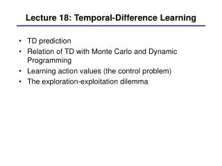
1. Chapter 6: Temporal Difference Learning • Introduce Temporal Difference (TD) learning • Focus first on policy evaluation, or prediction, methods • Then extend to control methods Objectives of this chapter: R. S. Sutton and A. G. Barto: Reinforcement Learning: An Introduction

2. TD Prediction Policy Evaluation (the prediction problem): for a given policy p, compute the state-value function Recall: target: the actual return after time t Must wait until the end of the episode target: an estimate of the return R. S. Sutton and A. G. Barto: Reinforcement Learning: An Introduction

3. T T T T T T T T T T T T T T T T T T T T Simple Monte Carlo R. S. Sutton and A. G. Barto: Reinforcement Learning: An Introduction

4. T T T T T T T T T T T T T T T T T T T T Simplest TD Method R. S. Sutton and A. G. Barto: Reinforcement Learning: An Introduction

5. T T T T T T T T T T cf. Dynamic Programming T T T R. S. Sutton and A. G. Barto: Reinforcement Learning: An Introduction

6. TD Bootstraps and Samples • Bootstrapping: update involves an estimate • MC does not bootstrap • DP bootstraps • TD bootstraps • Sampling: update does not involve an expected value • MC samples • DP does not sample • TD samples R. S. Sutton and A. G. Barto: Reinforcement Learning: An Introduction

7. Example: Driving Home R. S. Sutton and A. G. Barto: Reinforcement Learning: An Introduction

8. Driving Home • Changes recommended by Monte Carlo methods (a=1) • Changes recommended • by TD methods (a=1) R. S. Sutton and A. G. Barto: Reinforcement Learning: An Introduction

9. Advantages of TD Learning • TD methods do not require a model of the environment, only experience • TD, but not MC, methods can be fully incremental • You can learn before knowing the final outcome • Less memory • Less peak computation • You can learn without the final outcome • From incomplete sequences • Both MC and TD converge (under certain assumptions to be detailed later), but which is faster? R. S. Sutton and A. G. Barto: Reinforcement Learning: An Introduction

10. Random Walk Example Episodes terminate on either end with reward 0 (left) and 1 (right) • Values learned by TD(0) after • various numbers of episodes R. S. Sutton and A. G. Barto: Reinforcement Learning: An Introduction

11. TD and MC on the Random Walk • Data averaged over • 100 sequences of episodes R. S. Sutton and A. G. Barto: Reinforcement Learning: An Introduction

12. Optimality of TD(0) Batch Updating: train completely on a finite amount of data, e.g., train repeatedly on 10 episodes until convergence. Compute updates according to TD(0), but only update estimates after each complete pass through the data. For any finite Markov prediction task, under batch updating, TD(0) converges for sufficiently small a. Constant-a MC also converges under these conditions, but to a different answer! It converges to sample averages of the actual returns at each visited state. R. S. Sutton and A. G. Barto: Reinforcement Learning: An Introduction

13. Random Walk under Batch Updating • After each new episode, all previous episodes were treated as a batch, and algorithm was trained until convergence. All repeated 100 times. • TD seems to be better than MC, but MC gives optimum estimate of mean square error over the actual returns. So why TD seems better than the optimum? In what sense? R. S. Sutton and A. G. Barto: Reinforcement Learning: An Introduction

14. You are the Predictor Suppose you observe the following 8 episodes: A, 0, B, 0 B, 1 B, 1 B, 1 B, 1 B, 1 B, 1 B, 0 R. S. Sutton and A. G. Barto: Reinforcement Learning: An Introduction

15. You are the Predictor R. S. Sutton and A. G. Barto: Reinforcement Learning: An Introduction

16. You are the Predictor • The prediction that best matches the training data is V(A)=0 • This minimizes the mean-square-error on the training set • This is what a batch Monte Carlo method gets • If we consider the sequentiality of the problem, then we would set V(A)=.75 • This is correct for the maximum likelihood estimate of a Markov model generating the data • i.e, if we do a best fit Markov model, and assume it is exactly correct, and then compute what it predicts (how?) • This is called the certainty-equivalence estimate • This is what TD(0) gets R. S. Sutton and A. G. Barto: Reinforcement Learning: An Introduction

17. Learning An Action-Value Function R. S. Sutton and A. G. Barto: Reinforcement Learning: An Introduction

18. Sarsa: On-Policy TD Control Turn this into a control method by always updating the policy to be greedy with respect to the current estimate: The name SARSA comes from the sequence s(t) a(t) r(t+1) s(t+1) a(t+1) R. S. Sutton and A. G. Barto: Reinforcement Learning: An Introduction

19. Windy Gridworld undiscounted, episodic, reward = –1 until goal R. S. Sutton and A. G. Barto: Reinforcement Learning: An Introduction

20. Results of Sarsa on the Windy Gridworld R. S. Sutton and A. G. Barto: Reinforcement Learning: An Introduction

21. Results of Sarsa on the Windy Gridworld R. S. Sutton and A. G. Barto: Reinforcement Learning: An Introduction

22. Results of Sarsa on the Windy Gridworld % Example 6.5 % states are numbered from 1 to 70 according to raw and column index % matrix is scanned columnwise clear all; close all; % rewards r=0*(1:70)-1; r(53)=0; % next state for action - going north S_prime(1,1)=1; S_prime(1,2:70)=(1:69); S_prime(1,1:7:64)=(1:7:64); Spr=reshape(S_prime,7,10); % wind effect Spr(:,4:9)=[Spr(1,4:9); Spr(1:6,4:9)]; Spr(:,7:8)=[Spr(1,7:8); Spr(1:6,7:8)]; S_prime(1,:)=reshape(Spr,1,70); % next state for action - going east Spr=(8:70); Spr=reshape(Spr,7,9); Spr=[Spr Spr(:,9)]; % wind effect Spr(:,4:9)=[Spr(1,4:9); Spr(1:6,4:9)]; Spr(:,7:8)=[Spr(1,7:8); Spr(1:6,7:8)]; S_prime(2,:)=reshape(Spr,1,70); % next state for action - going south Spr=(1:70); Spr=reshape(Spr,7,10); Spr=[Spr(2:7,:); Spr(7,:)]; % wind effect Spr(:,4:9)=[Spr(1,4:9); Spr(1:6,4:9)]; Spr(1,4:9)=(22:7:57); Spr(:,7:8)=[Spr(1,7:8); Spr(1:6,7:8)]; S_prime(3,:)=reshape(Spr,1,70); % next state for action - going west Spr=(1:70); Spr=reshape(Spr,7,10); Spr=[Spr(:,1) Spr(:,1:9)]; % wind effect Spr(:,4:9)=[Spr(1,4:9); Spr(1:6,4:9)]; Spr(:,7:8)=[Spr(1,7:8); Spr(1:6,7:8)]; S_prime(4,:)=reshape(Spr,1,70); % initialize variables Qsa=zeros(4,70); alpha=0.9; epsi=0.1; gamma=0.9; num_episodes=170; t=1; R. S. Sutton and A. G. Barto: Reinforcement Learning: An Introduction

23. Results of Sarsa on the Windy Gridworld while s~=53 epsi=1/t; % take action a, observe r, s_pr s_pr=S_prime(a,s); % chose action a_pr from s_pr using epsilon greedy policy chose_policy_pr=rand>epsi; if chose_policy_pr [val,a_pr]=max(Qsa(:,s_pr)); random=[random 0]; else a_pr=ceil(rand*(1-eps)*4); random=[random 1]; end; % Bellman equation Qsa(a,s)=Qsa(a,s)+alpha*(-1+gamma*Qsa(a_pr,s_pr)-Qsa(a,s)); % the following selection works better % Qsa(a,s)=Qsa(a_pr,s_pr)-1; s=s_pr; a=a_pr; episode_size(episode)=episode_size(episode)+1; path=[path s]; t=t+1; end; %while s end; % repeat for each episode for episode=1:num_episodes epsi=1/t; % intitialize state s=4; % chose action a from s using epsilon greedy policy chose_policy=rand>epsi; if chose_policy [val,a]=max(Qsa(:,s)); else a=ceil(rand*(1-eps)*4); end; % repeat for each step of episode episode_size(episode)=0; path=[ ]; random=[ ]; R. S. Sutton and A. G. Barto: Reinforcement Learning: An Introduction

24. Results of Sarsa on the Windy Gridworld plot([0 cumsum(episode_size)],(0:num_episodes)); xlabel('Time step'); ylabel('Episode index'); title('Windy gridworld learning rate with eps=1/t, alpha=0.9'); figure(2) plot( episode_size(1:num_episodes)) xlabel('Episode index'); ylabel('Episode length in steps'); title('Windy gridworld learning rate with eps=1/t, alpha=0.9'); % determine the optimum policy for i=1:70 Optimum_policy(:,i)=(Qsa(:,i)==max(Qsa(:,i))); end; norm=sum(Optimum_policy); for i=1:70 Optimum_policy(:,i)=Optimum_policy(:,i)./norm(i); end % Optimum path % path = % Columns 1 through 13 % 11 18 25 31 37 43 50 57 64 65 66 67 68 % Columns 14 through 15 % 61 53 R. S. Sutton and A. G. Barto: Reinforcement Learning: An Introduction

25. Q-Learning: Off-Policy TD Control Different than in on-policy TD (SARSA) R. S. Sutton and A. G. Barto: Reinforcement Learning: An Introduction

26. Cliffwalking Sarsa Q-learning Reward for all moves –1 Falling off the cliff –100 • e-greedy, e = 0.1 R. S. Sutton and A. G. Barto: Reinforcement Learning: An Introduction

27. Actor-Critic Methods • Explicit representation of policy as well as value function • Minimal computation to select actions • Can learn an explicit stochastic policy • Can put constraints on policies • Appealing as psychological and neural models R. S. Sutton and A. G. Barto: Reinforcement Learning: An Introduction

28. Actor-Critic Details So with positive dthe preference for this action is increased and opposite R. S. Sutton and A. G. Barto: Reinforcement Learning: An Introduction

29. Striatum (Caudate nucleus) Nucleus accumbens VTA & Substantia Nigra (not shown) Amygdala Hippocampus Dopamine Neurons and TD Error W. Schultz et al. Universite de Fribourg R. S. Sutton and A. G. Barto: Reinforcement Learning: An Introduction

30. The CAR task • In the CAR task, a rat is trained that a conditioned stimulus(CS), such as a light or sound, precedes an unconditioned stimulus(US) such as an electric shock. Under normal conditions, the rat will learn to do two things: • First, it will learn to escape the shock by moving to the other side of the cage (for example). • Secondly, it will eventually learn that the CS predicts the shock, and the rat will then avoid the shock entirely by taking evasive action in response to the CS. R. S. Sutton and A. G. Barto: Reinforcement Learning: An Introduction

31. A computational model Following formal models of Reinforcement Learning (RL) (Sutton and Barto, 1998), we translate the CAR task into a Markov Decision Process (MDP). Each circle represents a different state the simulated rat can be in, and the arrows denote the outcome of each of the two possible actions. The shock of the US elicits a punishment of -1. The rat must learn to take the appropriate action in each state which minimises overall punishment. R. S. Sutton and A. G. Barto: Reinforcement Learning: An Introduction

32. R-Learning R-Learning is an off-policy control method for advanced RL when one neither discounts nor divides experience into distinct episodes. Instead try to find the maximum reward per time step. R. S. Sutton and A. G. Barto: Reinforcement Learning: An Introduction

33. Average Reward Per Time Step in R-Learning the same for each state if ergodic i.e. nonzero probability of reaching any state This is a transient value declining to zero as all states reach their final average reward r R. S. Sutton and A. G. Barto: Reinforcement Learning: An Introduction

34. Access-Control Queuing Task Apply R-learning • n servers • Customers have four different priorities, which pay reward of 1, 2, 3, or 4, if served • At each time step, customer at head of queue is accepted (assigned to a server) or removed from the queue • Proportion of randomly distributed high priority customers in queue is h • Busy server becomes free with probability p on each time step • Statistics of arrivals and departures are unknown n=10, h=.5, p=.06 R. S. Sutton and A. G. Barto: Reinforcement Learning: An Introduction

35. Afterstates • Usually, a state-value function evaluates states in which the agent can take an action. • But sometimes it is useful to evaluate states after agent has acted, as in tic-tac-toe. • Why is this useful? We do not know the opponent’s response so determining the state value is difficult • Action-value also do not work since different states and actions may result in the same board position • What is this in general? R. S. Sutton and A. G. Barto: Reinforcement Learning: An Introduction

36. Summary • TD prediction • Introduced one-step tabular model-free TD methods • Extend prediction to control by employing some form of GPI • On-policy control: Sarsa • Off-policy control: Q-learning and R-learning • These methods bootstrap and sample, combining aspects of DP and MC methods R. S. Sutton and A. G. Barto: Reinforcement Learning: An Introduction