Download
1 / 93
970 likes | 1.01k Views
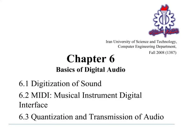
Iran University of Science and Technology, Computer Engineering Department, Fall 2008 (1387). Chapter 6 Basics of Digital Audio. 6.1 Digitization of Sound 6.2 MIDI: Musical Instrument Digital Interface 6.3 Quantization and Transmission of Audio. 6.1 Digitization of Sound. What is Sound?

E N D
Iran University of Science and Technology,Computer Engineering Department, Fall 2008 (1387) Chapter 6Basics of Digital Audio 6.1 Digitization of Sound 6.2 MIDI: Musical Instrument Digital Interface 6.3 Quantization and Transmission of Audio
6.1 Digitization of Sound • What is Sound? • • Sound is a wave phenomenon like light, but is macroscopic and involves molecules of air being compressed and expanded under the action of some physical device. • (a) For example, a speaker in an audio system vibrates back and forth and produces a longitudinal pressure wave that we perceive as sound. • (b) Since sound is a pressure wave, it takes on continuous values, as opposed to digitized ones. Multimedia Systems (eadeli@iust.ac.ir)
(c) Even though such pressure waves are longitudinal, they still have ordinary wave properties and behaviors, such as reflection (bouncing), refraction (change of angle when entering a medium with a different density) and diffraction (bending around an obstacle). • (d) If we wish to use a digital version of sound waves we must form digitized representations of audio information. Multimedia Systems (eadeli@iust.ac.ir)
Digitization • • Digitization means conversion to a stream of numbers, and preferably these numbers should be integers for efficiency. • • Fig. 6.1 shows the 1-dimensional nature of sound: amplitude values depend on a 1D variable, time. (And note that images depend instead on a 2D set of variables, x and y). Multimedia Systems (eadeli@iust.ac.ir)
Fig. 6.1: An analog signal: continuous measurement of pressure wave. Multimedia Systems (eadeli@iust.ac.ir)
• The graph in Fig. 6.1 has to be made digital in both time and amplitude. To digitize, the signal must be sampled in each dimension: in time, and in amplitude. • (a) Sampling means measuring the quantity we are interested in, usually at evenly-spaced intervals. • (b) The first kind of sampling, using measurements only at evenly spaced time intervals, is simply called, sampling. The rate at which it is performed is called the sampling frequency (see Fig. 6.2(a)). • (c) For audio, typical sampling rates are from 8 kHz (8,000 samples per second) to 48 kHz. This range is determined by the Nyquist theorem, discussed later. • (d) Sampling in the amplitude or voltage dimension is called quantization. Fig. 6.2(b) shows this kind of sampling. Multimedia Systems (eadeli@iust.ac.ir)
Fig. 6.2: Sampling and Quantization. (a): Sampling the analog signal in the time dimension. (b): Quantization is sampling the analog signal in the amplitude dimension. (a) (b) Multimedia Systems (eadeli@iust.ac.ir)
• Thus to decide how to digitize audio data we need to answer the following questions: • What is the sampling rate? • 2. How finely is the data to be quantized, and is quantization uniform? • 3. How is audio data formatted? (file format) Multimedia Systems (eadeli@iust.ac.ir)
Nyquist Theorem • • Signals can be decomposed into a sum of sinusoids. Fig. 6.3 shows how weighted sinusoids can build up quite a complex signal. Multimedia Systems (eadeli@iust.ac.ir)
Fig. 6.3: Building up a complex signal by superposing sinusoids Multimedia Systems (eadeli@iust.ac.ir)
• The Nyquist theorem states how frequently we must sample in time to be able to recover the original sound. • (a) Fig. 6.4(a) shows a single sinusoid: it is a single, pure, frequency (only electronic instruments can create such sounds). • (b) If sampling rate just equals the actual frequency, Fig. 6.4(b) shows that a false signal is detected: it is simply a constant, with zero frequency. • (c) Now if sample at 1.5 times the actual frequency, Fig. 6.4(c) shows that we obtain an incorrect (alias) frequency that is lower than the correct one — it is half the correct one (the wavelength, from peak to peak, is double that of the actual signal). • (d) Thus for correct sampling we must use a sampling rate equal to at least twice the maximum frequency content in the signal. This rate is called the Nyquist rate. Multimedia Systems (eadeli@iust.ac.ir)
Fig. 6.4: Aliasing. (a): A single frequency. (b): Sampling at exactly the frequency produces a constant. (c): Sampling at 1.5 times per cycle produces an alias perceived frequency. Multimedia Systems (eadeli@iust.ac.ir)
Aliasing in an Image Signal Sampling Without Aliasing Sampling With Aliasing Multimedia Systems (eadeli@iust.ac.ir)
• Nyquist Theorem: If a signal is band-limited, i.e., there is a lower limit f1 and an upper limit f2of frequency components in the signal, then the sampling rate should be at least 2(f2 − f1). • • Nyquist frequency: half of the Nyquist rate. • – Since it would be impossible to recover frequencies higher than Nyquist frequency in any event, most systems have an antialiasing filter that restricts the frequency content in the input to the sampler to a range at or below Nyquist frequency. • • The relationship among the Sampling Frequency, True Frequency, and the Alias Frequency is as follows: • falias= fsampling− ftrue, for ftrue< fsampling< 2 × ftrue(6.1) Multimedia Systems (eadeli@iust.ac.ir)
Signal to Noise Ratio (SNR) • • The ratio of the power of the correct signal and the noise is called the signal to noise ratio (SNR) — a measure of the quality of the signal. • • The SNR is usually measured in decibels (dB), where 1 dB is a tenth of a bel. The SNR value, in units of dB, is defined in terms of base-10 logarithms of squared voltages, as follows: • (6.2) Multimedia Systems (eadeli@iust.ac.ir)
The power in a signal is proportional to the square of the voltage. For example, if the signal voltage Vsignalis 10 times the noise, then the SNR is 20 ∗ log10(10) = 20dB. • b) In terms of power, if the power from ten violins is ten times that from one violin playing, then the ratio of power is 10dB, or 1B. Multimedia Systems (eadeli@iust.ac.ir)
• The usual levels of sound we hear around us are described in terms of decibels, as a ratio to the quietest sound we are capable of hearing. Table 6.1 shows approximate levels for these sounds. • Table 6.1: Magnitude levels of common sounds, in decibels Multimedia Systems (eadeli@iust.ac.ir)
Signal to Quantization Noise Ratio (SQNR) • • Aside from any noise that may have been present in the original analog signal, there is also an additional error that results from quantization. • (a) If voltages are actually in 0 to 1 but we have only 8 bits in which to store values, then effectively we force all continuous values of voltage into only 256 different values. • (b) This introduces a roundoff error. It is not really “noise”. Nevertheless it is called quantization noise (or quantization error). Multimedia Systems (eadeli@iust.ac.ir)
• The quality of the quantization is characterized by the Signal to Quantization Noise Ratio (SQNR). • Quantization noise: the difference between the actual value of the analog signal, for the particular sampling time, and the nearest quantization interval value. • (b) At most, this error can be as much as half of the interval. Multimedia Systems (eadeli@iust.ac.ir)
(c) For a quantization accuracy of N bits per sample, the SQNR can be simply expressed: • (6.3) • • Notes: • We map the maximum signal to 2N−1 − 1 (≃ 2N−1) and the most negative signal to −2N−1. • (b) Eq. (6.3) is the Peak signal-to-noise ratio, PSQNR: peak signal and peak noise. Multimedia Systems (eadeli@iust.ac.ir)
(c) The dynamic range is the ratio of maximum to minimum absolute values of the signal: Vmax/Vmin. The max abs. value Vmax gets mapped to 2N−1 − 1; the min abs. value Vmin gets mapped to 1. Vminis the smallest positive voltage that is not masked by noise. The most negative signal, −Vmax, is mapped to −2N−1. • (d) The quantization interval is ΔV=(2Vmax)/2N, since there are 2N intervals. The whole range Vmax down to (Vmax − ΔV/2) is mapped to 2N−1 − 1. • (e) The maximum noise, in terms of actual voltages, is half the quantization interval: ΔV/2 = Vmax/2N. Multimedia Systems (eadeli@iust.ac.ir)
Linear and Non-linear Quantization • • Linear format: samples are typically stored as uniformly quantized values. • • Non-uniform quantization: set up more finely-spaced levels where humans hear with the most acuity. • – Weber’s Law stated formally says that equally perceived differences have values proportional to absolute levels: • ΔResponse ∝ ΔStimulus/Stimulus (6.5) • – Inserting a constant of proportionality k, we have a differential equation that states: • dr = k (1/s) ds (6.6) • with response r and stimulus s. Multimedia Systems (eadeli@iust.ac.ir)
– Integrating, we arrive at a solution • r = k ln s + C (6.7) • with constant of integration C. • Stated differently, the solution is • r = kln(s/s0) (6.8) • s0 = the lowest level of stimulus that causes a response (r = 0 when s = s0). • • Nonlinear quantization works by first transforming an analog signal from the raw s space into the theoretical r space, and then uniformly quantizing the resulting values. • • Such a law for audio is called μ-law encoding, (or u-law). A very similar rule, called • A-law, is used in telephony in Europe. • • The equations for these very similar encodings are as follows: Multimedia Systems (eadeli@iust.ac.ir)
μ-law: • (6.9) • A-law: • (6.10) • • Fig. 6.6 shows these curves. The parameter μ is set to μ = 100 or μ = 255; the parameter A for the A-law encoder is usually set to A = 87.6. Multimedia Systems (eadeli@iust.ac.ir)
Fig. 6.6: Nonlinear transform for audio signals • • The μ-law in audio is used to develop a nonuniform quantization rule for sound: uniform quantization of r gives finer resolution in s at the quiet end. Multimedia Systems (eadeli@iust.ac.ir)
Audio Filtering • • Prior to sampling and AD conversion, the audio signal is also usually filtered to remove unwanted frequencies. The frequencies kept depend on the application: • (a) For speech, typically from 50Hz to 10kHz is retained, and other frequencies • are blocked by the use of a band-pass filter that screens out lower and higher frequencies. • (b) An audio music signal will typically contain from about 20Hz up to 20kHz. • (c) At the DA converter end, high frequencies may reappear in the output — because of sampling and then quantization, smooth input signal is replaced by a series of step functions containing all possible frequencies. • (d) So at the decoder side, a lowpassfilter is used after the DA circuit. Multimedia Systems (eadeli@iust.ac.ir)
Audio Quality vs. Data Rate • • The uncompressed data rate increases as more bits are used for quantization. Stereo: double the bandwidth. to transmit a digital audio signal. • Table 6.2: Data rate and bandwidth in sample audio applications Multimedia Systems (eadeli@iust.ac.ir)
Synthetic Sounds • FM (Frequency Modulation): one approach to generating synthetic sound: • (6.11) Multimedia Systems (eadeli@iust.ac.ir)
π π • Fig. 6.7: Frequency Modulation. (a): A single frequency. (b): Twice the frequency. (c): Usually, FM is carried out using a sinusoid argument to a sinusoid. (d): A more complex form arises from a carrier frequency, 2πt and a modulating frequency 4πt cosine inside the sinusoid. π π π Multimedia Systems (eadeli@iust.ac.ir)
2. Wave Table synthesis: A more accurate way of generating sounds from digital signals. Also known, simply, as sampling. • In this technique, the actual digital samples of sounds from real instruments are stored. Since wave tables are stored in memory on the sound card, they can be manipulated by software so that sounds can be combined, edited, and enhanced. Multimedia Systems (eadeli@iust.ac.ir)
6.2 MIDI: Musical Instrument Digital Interface • • Use the sound card’s defaults for sounds: ⇒ use a simple scripting language and hardware setup called MIDI. • • MIDI Overview • (a) MIDI is a scripting language — it codes “events” that stand for the production of sounds. E.g., a MIDI event might include values for the pitch of a single note, its duration, and its volume. • (b) MIDI is a standard adopted by the electronic music industry for controlling devices, such as synthesizers and sound cards, that produce music. Multimedia Systems (eadeli@iust.ac.ir)
(c) The MIDI standard is supported by most synthesizers, so sounds created on one synthesizer can be played and manipulated on another synthesizer and sound reasonably close. • (d) Computers must have a special MIDI interface, but this is incorporated into most sound cards. The sound card must also have both D/A and A/D converters. Multimedia Systems (eadeli@iust.ac.ir)
MIDI Concepts • • MIDI channels are used to separate messages. • (a) There are 16 channels numbered from 0 to 15. The channel forms the last 4 bits (the least significant bits) of the message. • (b) Usually a channel is associated with a particular instrument: e.g., channel 1 is the piano, channel 10 is the drums, etc. • (c) Nevertheless, one can switch instruments midstream, if desired, and associate another instrument with any channel. Multimedia Systems (eadeli@iust.ac.ir)
• System messages • (a) Several other types of messages, e.g. a general message for all instruments indicating a change in tuning or timing. • (b) If the first 4 bits are all 1s, then the message is interpreted as a system common message. • • The way a synthetic musical instrument responds to a MIDI message is usually by simply ignoring any play sound message that is not for its channel. • – If several messages are for its channel, then the instrument responds, provided it is multi-voice, i.e., can play more than a single note at once. Multimedia Systems (eadeli@iust.ac.ir)
• It is easy to confuse the term voice with the term timbre — the latter is MIDI terminology for just what instrument that is trying to be emulated, e.g. a piano as opposed to a violin: it is the quality of the sound. • (a) An instrument (or sound card) that is multi-timbralis one that is capable of playing many different sounds at the same time, e.g., piano, brass, drums, etc. • (b) On the other hand, the term voice, while sometimes used by musicians to mean the same thing as timbre, is used in MIDI to mean every different timbre and pitch that the tone module can produce at the same time. • • Different timbres are produced digitally by using a patch — the set of control settings that define a particular timbre. Patches are often organized into databases, called banks. Multimedia Systems (eadeli@iust.ac.ir)
• General MIDI: A standard mapping specifying what instruments (what patches) will be associated with what channels. • (a) In General MIDI, channel 10 is reserved for percussion instruments, and there are 128 patches associated with standard instruments. • (b) For most instruments, a typical message might be a Note On message (meaning, e.g., a keypress and release), consisting of what channel, what pitch, and what “velocity” (i.e., volume). • (c) A Note On message consists of “status” byte — which channel, what pitch — followed by two data bytes. It is followed by a Note Off message, which also has a pitch (which note to turn off) and a velocity (often set to zero). Multimedia Systems (eadeli@iust.ac.ir)
• The data in a MIDI status byte is between 128 and 255; each of the data bytes is between 0 and 127. Actual MIDI bytes are 10-bit, including a 0 start and 0 stop bit. • Fig. 6.8: Stream of 10-bit bytes; for typical MIDI messages, these consist of {Status byte, Data Byte, Data Byte} = {Note On, Note Number, Note Velocity} Multimedia Systems (eadeli@iust.ac.ir)
• A MIDI device often is capable of programmability, and also can change the envelope describing how the amplitude of a sound changes over time. • • Fig. 6.9 shows a model of the response of a digital instrument to a Note On message: • Fig. 6.9: Stages of amplitude versus time for a music note Multimedia Systems (eadeli@iust.ac.ir)
Hardware Aspects of MIDI • • The MIDI hardware setup consists of a 31.25 kbps serial connection. Usually, MIDI-capable units are either Input devices or Output devices, not both. • • A traditional synthesizer is shown in Fig. 6.10: • Fig. 6.10: A MIDI synthesizer Multimedia Systems (eadeli@iust.ac.ir)
• The physical MIDI ports consist of 5-pin connectors for IN and OUT, as well as a third connector called THRU. • MIDI communication is half-duplex. • (b) MIDI IN is the connector via which the device receives all MIDI data. • (c) MIDI OUT is the connector through which the device transmits all the MIDI data it generates itself. • (d) MIDI THRU is the connector by which the device echoes the data it receives from MIDI IN. Note that it is only the MIDI IN data that is echoed by MIDI THRU — all the data generated by the device itself is sent via MIDI OUT. Multimedia Systems (eadeli@iust.ac.ir)
• A typical MIDI sequencer setup is shown in Fig. 6.11: Fig. 6.11: A typical MIDI setup Multimedia Systems (eadeli@iust.ac.ir)
Structure of MIDI Messages • • MIDI messages can be classified into two types: channel messages and system messages, as in Fig. 6.12: • Fig. 6.12: MIDI message taxonomy Multimedia Systems (eadeli@iust.ac.ir)
• A. Channel messages: can have up to 3 bytes: • a) The first byte is the status byte (the opcode, as it were); has its most significant bit set to 1. • b) The 4 low-order bits identify which channel this message belongs to (for 16 possible channels). • c) The 3 remaining bits hold the message. For a data byte, the most significant bit is set to 0. • • A.1. Voice messages: • a) This type of channel message controls a voice, i.e., sends information specifying which note to play or to turn off, and encodes key pressure. • b) Voice messages are also used to specify controller effects such as sustain, vibrato, tremolo, and the pitch wheel. • c) Table 6.3 lists these operations. Multimedia Systems (eadeli@iust.ac.ir)
Table 6.3: MIDI voice messages • (** &H indicates hexadecimal, and ‘n’ in the status byte hex value stands for a channel number. All values are in 0..127 except Controller number, which is in 0..120) Multimedia Systems (eadeli@iust.ac.ir)
• A.2. Channel mode messages: • a) Channel mode messages: special case of the Control Change message → opcode B (the message is &HBn, or 1011nnnn). • b) However, a Channel Mode message has its first data byte in 121 through 127 (&H79–7F). • c) Channel mode messages determine how an instrument processes MIDI voice messages: respond to all messages, respond just to the correct channel, don’t respond at all, or go over to local control of the instrument. • d) The data bytes have meanings as shown in Table 6.4. Multimedia Systems (eadeli@iust.ac.ir)
Table 6.4: MIDI mode messages Multimedia Systems (eadeli@iust.ac.ir)
• B. System Messages: • a) System messages have no channel number — commands that are not channel specific, such as timing signals for synchronization, positioning information in pre-recorded MIDI sequences, and detailed setup information for the destination device. • b) Opcodes for all system messages start with &HF. • c) System messages are divided into three classifications, according to their use: Multimedia Systems (eadeli@iust.ac.ir)
B.1. System common messages: relate to timing or positioning. • Table 6.5: MIDI System Common messages. Multimedia Systems (eadeli@iust.ac.ir)
B.2. System real-time messages: related to synchronization. • Table 6.6: MIDI System Real-Time messages. Multimedia Systems (eadeli@iust.ac.ir)
B.3. System exclusive message: included so that the MIDI • standard can be extended by manufacturers. • a) After the initial code, a stream of any specific messages can be inserted that apply to their own product. • b) A System Exclusive message is supposed to be terminated by a terminator byte &HF7, as specified in Table 6. • c) The terminator is optional and the data stream may simply be ended by sending the status byte of the next message. Multimedia Systems (eadeli@iust.ac.ir)