Download
1 / 66
870 likes | 1.45k Views
Chapter 6 Basics of Digital Audio. 6.1 Digitization of Sound 6.2 MIDI: Musical Instrument Digital Interface 6.3 Quantization and Transmission of Audio 6.4 Further Exploration. What is sound?.

E N D
Chapter 6Basics of Digital Audio 6.1 Digitization of Sound 6.2 MIDI: Musical Instrument Digital Interface 6.3 Quantization and Transmission of Audio 6.4 Further Exploration Li & Drew
What is sound? • • Sound is a wave phenomenon like light, but is macroscopic and involves molecules of air being compressed and expanded under the action of some physical device. • (a) For example, a speaker in an audio system vibrates back and forth and produces a longitudinal pressure wave that we perceive as sound. • (b) Since sound is a pressure wave, it takes on continuous values, as opposed to digitized ones. Li & Drew Physics of Sound
Sound Wave Li & Drew
How does the ear work? As the sound waves enter the ear, the ear canal increases the loudness of those pitches that make it easier to understand speech and protects the eardrum - a flexible, circular membrane which vibrates when touched by sound waves. Li & Drew
How does the ear work? As the sound waves enter the ear, the ear canal increases the loudness of those pitches that make it easier to understand speech and protects the eardrum - a flexible, circular membrane which vibrates when touched by sound waves. The sound vibrations continue their journey into the middle ear, which contains three tiny bones called the ossicles, which are also known as the hammer, anvil and stirrup. These bones form the bridge from the eardrum into the inner ear. They increase and amplify the sound vibrations even more, before safely transmitting them on to the inner ear via the oval window. Li & Drew
How does the ear work? As the sound waves enter the ear, the ear canal increases the loudness of those pitches that make it easier to understand speech and protects the eardrum - a flexible, circular membrane which vibrates when touched by sound waves. The sound vibrations continue their journey into the middle ear, which contains three tiny bones called the ossicles, which are also known as the hammer, anvil and stirrup. These bones form the bridge from the eardrum into the inner ear. They increase and amplify the sound vibrations even more, before safely transmitting them on to the inner ear via the oval window. The Inner Ear (cochlea), houses a system of tubes filled with a watery fluid. As the sound waves pass through the oval window the fluid begins to move, setting tiny hair cells in motion. In turn, these hairs transform the vibrations into electrical impulses that travel along the auditory nerve to the brain itself. link Li & Drew
Hearing by Age Group Article Mosquito Ringtones
(c) Even though such pressure waves are longitudinal, they still have ordinary wave properties and behaviors, such as reflection (bouncing), refraction (change of angle when entering a medium with a different density) and diffraction (bending around an obstacle). • (d) If we wish to use a digital version of sound waves we must form digitized representations of audio information. • Link to physical description of sound waves. Li & Drew
Digitization • • Digitization means conversion to a stream of numbers, and preferably these numbers should be integers for efficiency. Li & Drew
An analog signal: continuous measurement of pressure wave. • Sound is 1-dimensional (amplitude values depend on a 1D variable, time) as opposed to images which are 2D (x,y) Li & Drew
• The graph in Fig. 6.1 has to be made digital in both time and amplitude. To digitize, the signal must be sampled in each dimension: in time, and in amplitude. • (a) Sampling means measuring the quantity we are interested in, usually at evenly-spaced intervals. • (b) The first kind of sampling, using measurements only at evenly spaced time intervals, is simply called, sampling. The rate at which it is performed is called the sampling frequency. • (c) For audio, typical sampling rates are from 8 kHz (8,000 samples per second) to 48 kHz. This range is determined by the Nyquist theorem, discussed later. • (d) Sound is a continuous signal (measurement of pressure). Sampling in the amplitude or voltage dimension is called quantization. We quantize so that we can represent the signal as a discrete set of values. Li & Drew
Fig. 6.2: Sampling and Quantization. (a): Sampling the analog signal in the time dimension. (b): Quantization is sampling the analog signal in the amplitude dimension. (a) (b) Li & Drew
Building up a complex signal by superposing sinusoids Signals can be decomposed into a weighted sum of sinusoids: Li & Drew
• Whereas frequency is an absolute measure, pitch is generally relative — a perceptual subjective quality of sound. • (a) Pitch and frequency are linked by setting the note A above middle C to exactly 440 Hz. • (b) An octave above that note takes us to another A note. An octave corresponds to doubling the frequency. Thus with the middle “A” on a piano (“A4” or “A440”) set to 440 Hz, the next “A” up is at 880 Hz, or one octave above. • (c) Harmonics: any series of musical tones whose frequencies are integral multiples of the frequency of a fundamental tone: Fig. 6. • (d) If we allow non-integer multiples of the base frequency, we allow non-“A” notes and have a more complex resulting sound. Demo in Matlab Li & Drew
• To decide how to digitize audio data we need to answer the following questions: • What is the sampling rate? • 2. How finely is the data to be quantized, and is quantization uniform? • 3. How is audio data formatted? (file format) Li & Drew
• The Nyquist theorem states how frequently we must sample in time to be able to recover the original sound. • (a) Fig. 6.4(a) shows a single sinusoid: it is a single, pure, frequency (only electronic instruments can create such sounds). • (b) If sampling rate just equals the actual frequency, Fig. 6.4(b) shows that a false signal is detected: it is simply a constant, with zero frequency. • (c) Now if sample at 1.5 times the actual frequency, Fig. 6.4(c) shows that we obtain an incorrect (alias) frequency that is lower than the correct one — it is half the correct one (the wavelength, from peak to peak, is double that of the actual signal). • (d) Thus for correct sampling we must use a sampling rate equal to at least twice the maximum frequency content in the signal. This rate is called the Nyquist rate. Li & Drew
Fig. 6.4: Aliasing. (a): A single frequency. (b): Sampling at exactly the frequency produces a constant. (c): Sampling at 1.5 times per cycle produces an alias perceived frequency. Li & Drew
• Nyquist Theorem: If a signal is band-limited, i.e., there is a lower limit f1 and an upper limit f2of frequency components in the signal, then the sampling rate should be at least 2(f2 − f1). • • Nyquist frequency: half of the Nyquist rate. • – Since it would be impossible to recover frequencies higher than Nyquist frequency in any event, most systems have an antialiasing filter that restricts the frequency content in the input to the sampler to a range at or below Nyquist frequency. Li & Drew
Aliasing • The relationship among the Sampling Frequency, • True Frequency, and the Alias Frequency is as • follows: • falias = fsampling − ftrue, for ftrue < fsampling < 2 × ftrue • If true freq is 5.5 kHz and sampling freq is 8 kHz. • Then what is the alias freq? Li & Drew
Signal to Noise Ratio (SNR) • • The ratio of the power of the correct signal and the noise is called the signal to noise ratio (SNR) — a measure of the quality of the signal. • • The SNR is usually measured in decibels (dB), where 1 dB is a tenth of a bel. The SNR value, in units of dB, is defined in terms of base-10 logarithms of squared amplitudes, as follows: • (6.2) Li & Drew
For example, if the signal amplitude Asignalis 10 times the noise, then the SNR is • 20 ∗ log10(10) = 20dB. • b) dB always defined in terms of a ratio. Li & Drew
• The usual levels of sound we hear around us are described in terms of decibels, as a ratio to the quietest sound we are capable of hearing. Table 6.1 shows approximate levels for these sounds. • Table 6.1: Magnitude levels of common sounds, in decibels Li & Drew
Merits of dB • * The decibel's logarithmic nature means that a very large range of ratios can be represented by a convenient number. This allows one to clearly visualize huge changes of some quantity. • * The mathematical properties of logarithms mean that the overall decibel gain of a multi-component system (such as consecutive amplifiers) can be calculated simply by summing the decibel gains of the individual components, rather than needing to multiply amplification factors. Essentially this is because log(A × B × C × ...) = log(A) + log(B) + log(C) + … • * The human perception of sound is such that a doubling of actual intensity causes perceived intensity to always increase by the same amount, irrespective of the original level. The decibel's logarithmic scale, in which a doubling of power or intensity always causes an increase of approximately 3 dB, corresponds to this perception. Li & Drew
Signal to Quantization Noise Ratio (SQNR) • • Aside from any noise that may have been present in the original analog signal, there is also an additional error that results from quantization. • (a) If voltages are actually in 0 to 1 but we have only 8 bits in which to store values, then effectively we force all continuous values of voltage into only 256 different values. • (b) This introduces a roundoff error. It is not really “noise”. Nevertheless it is called quantization noise (or quantization error). Li & Drew
• The quality of the quantization is characterized by the Signal to Quantization Noise Ratio (SQNR). • Quantization noise: the difference between the actual value of the analog signal, for the particular sampling time, and the nearest quantization interval value. • (b) At most, this error can be as much as half of the interval. Li & Drew
(c) For a quantization accuracy of N bits per sample, the SQNR can be simply expressed: • (6.3) • • Notes: • We map the maximum signal to 2N−1 − 1 (≃ 2N−1) and the most negative signal to −2N−1. • (b) Eq. (6.3) is the Peak signal-to-noise ratio, PSQNR: peak signal and peak noise. Li & Drew
(c) For a quantization accuracy of N bits per sample, the SQNR can be simply expressed: • (6.3) • • Notes: • We map the maximum signal to 2N−1 − 1 (≃ 2N−1) and the most negative signal to −2N−1. • (b) Eq. (6.3) is the Peak signal-to-noise ratio, PSQNR: peak signal and peak noise. In the worst case Li & Drew
Linear and Non-linear Quantization • • Linear format: samples are typically stored as uniformly quantized values. • • Non-uniform quantization: set up more finely-spaced levels where humans hear with the most acuity. • Nonlinear quantization works by first transforming an analog signal from the raw s space into the theoretical r space, and then uniformly quantizing the resulting values. • • Such a law for audio is called μ-law encoding. A very similar rule, called A-law, is used in telephony in Europe. Li & Drew
Fig. 6.6: Nonlinear transform for audio signals • • The μ-law in audio is used to develop a nonuniform quantization rule for sound: uniform quantization of r gives finer resolution in s at the quiet end (s/sp near 0). Transformed signal Current signal value / peak signal value Li & Drew
Values in s get mapped to values in r non-uniformly. “Perceptual coder” – allocates more bits to intervals for which a small change produces a large change in perception. • Fig. 6.6: Nonlinear transform for audio signals • • The μ-law in audio is used to develop a nonuniform quantization rule for sound: uniform quantization of r gives finer resolution in s at the quiet end (s/sp near 0). Transformed signal Current signal value / peak signal value Li & Drew
Quantization • Matlab demo Li & Drew
Audio Filtering • • Prior to sampling and AD conversion, the audio signal is also usually filtered to remove unwanted frequencies. The frequencies kept depend on the application: • (a) For speech, typically from 50Hz to 10kHz is retained, and other frequencies • are blocked by the use of a band-pass filter that screens out lower and higher frequencies. • (b) An audio music signal will typically contain from about 20Hz up to 20kHz. • (c) At the DA converter end, high frequencies may reappear in the output — because of sampling and then quantization. • (d) So at the decoder side, a lowpass filter is used after the DA circuit. • Next class we’ll see how to create filters in matlab and apply them to audio signals! Li & Drew
Audio Quality vs. Data Rate • • The uncompressed data rate increases as more bits are used for quantization. Stereo: double the bandwidth. to transmit a digital audio signal. • Table 6.2: Data rate and bandwidth in sample audio applications Li & Drew
Digital -> Analog • Digitized sound must be converted to analog for us to hear it. • Two different approaches • FM • WaveTable Li & Drew
Synthetic Sounds • FM (Frequency Modulation): one approach to generating synthetic sound: A(t) specifies overall loudness over time specifies the carrier frequency specifies the modulating frequency I(t) produces a feeling of harmonics (overtones) by changing the amount of the modulating frequency heard. Specify time-shifts for a more interesting sound Li & Drew
π π • Fig. 6.7: Frequency Modulation. (a): A single frequency. (b): Twice the frequency. (c): Usually, FM is carried out using a sinusoid argument to a sinusoid. (d): A more complex form arises from a carrier frequency, 2πt and a modulating frequency 4πt cosine inside the sinusoid. π π π Li & Drew
2. Wave Table synthesis: A more accurate way of generating sounds from digital signals. Also known, simply, as sampling. • In this technique, the actual digital samples of sounds from real instruments are stored. Since wave tables are stored in memory on the sound card, they can be manipulated by software so that sounds can be combined, edited, and enhanced. • → Link to details. Li & Drew
6.2 MIDI: Musical Instrument Digital Interface • • MIDI Overview • (a) MIDI is a protocol adopted by the electronic music industry in the early 80s for controlling devices, such as synthesizers and sound cards, that produce music and allowing them to communicate with each other. • (b) MIDI is a scripting language — it codes “events” that stand for the production of sounds. E.g., a MIDI event might include values for the pitch of a single note, its duration, and its volume. Li & Drew
(c) The MIDI standard is supported by most synthesizers, so sounds created on one synthesizer can be played and manipulated on another synthesizer and sound reasonably close. • (d) Computers must have a special MIDI interface, but this is incorporated into most sound cards. • (3) A MIDI file consists of a sequence of MIDI instructions (messages). So, would be quite small in comparison to a standard audio file. Li & Drew
MIDI Concepts • • MIDI channels are used to separate messages. • (a) There are 16 channels numbered from 0 to 15. The channel forms the last 4 bits (the least significant bits) of the message. • (b) Usually a channel is associated with a particular instrument: e.g., channel 1 is the piano, channel 10 is the drums, etc. • (c) Nevertheless, one can switch instruments midstream, if desired, and associate another instrument with any channel. Li & Drew
• System messages • Several other types of messages, e.g. a general message for all instruments indicating a change in tuning or timing. • • The way a synthetic musical instrument responds to a MIDI message is usually by simply ignoring any play sound message that is not for its channel. • – If several messages are for its channel (say play multiple notes on the piano), then the instrument responds, provided it is multi-voice, i.e., can play more than a single note at once (as opposed to violins). Li & Drew
• General MIDI: A standard mapping specifying what instruments will be associated with what channels. • (a) For most instruments, a typical message might be a Note On message (meaning, e.g., a keypress and release), consisting of what channel, what pitch, and what “velocity” (i.e., volume). • (b) For percussion instruments, however, the pitch data means which kind of drum. • (c) A Note On message consists of “status” byte — which channel, what pitch — followed by two data bytes. It is followed by a Note Off message, which also has a pitch (which note to turn off) and a velocity (often set to zero). Li & Drew
• The data in a MIDI status byte is between 128 and 255; each of the data bytes is between 0 and 127. Actual MIDI bytes are 10-bit, including a 0 start and 0 stop bit. • Fig. 6.8 Li & Drew
• A MIDI device often is capable of programmability, and also can change the envelope describing how the amplitude of a sound changes over time. • • Fig. 6.9 shows a model of the response of a digital instrument to a Note On message: • Fig. 6.9: Stages of amplitude versus time for a music note Li & Drew
6.3 Quantization and Transmission of Audio • • Coding of Audio: Quantization and transformation of data are collectively known as coding of the data. • a) For audio, the μ-law technique for companding audio signals is usually combined with an algorithm that exploits the temporal redundancy present in audio signals. • b) Encoding Differences in signals between the present and a past time can reduce the size of signal values into a much smaller range. • c) The result of reducing the variance of values is that lossless compression methods produce a bitstream with shorter bit lengths for more likely values. Li & Drew
• Every compression scheme has three stages: • A. The input data is transformed to a new representation that is easier or more efficient to compress. • B. We may introduce loss of information. Quantization is the main lossy step ⇒ we use a limited number of reconstruction levels, fewer than in the original signal. • C. Coding. Assign a codeword to each output level or symbol. Li & Drew
Pulse Code Modulation (PCM) • • The basic techniques for creating digital signals from analog signals are sampling and quantization. • • Quantization consists of selecting breakpoints in magnitude, and then re-mapping any value within an interval to one of the representative output levels. Li & Drew
Fig. 6.2: Sampling and Quantization. (a) (b) Li & Drew
Fig. 6.6: Nonlinear transform for audio signals • The μ-law in audio is used to develop a nonuniform quantization rule for sound: uniform quantization of r gives finer resolution in s at the quiet end (s/sp near 0). • Encode in this non-uniform space - can use fewer quantization levels for same perceptual quality (saw this in matlab demo). Transformed signal Current signal value / peak signal value Li & Drew
PCM in Speech Compression • • Assuming a bandwidth for speech from about 50 Hz to about 10 kHz, the Nyquist rate would dictate a sampling rate of 20 kHz. • (a) Using uniform quantization, the minimum sample size we could get away with would likely be about 12 bits. Hence for mono speech transmission the bit-rate would be 240 kbps. • (b) With non-uniform quantization, we can reduce the sample size down to about 8 bits with the same perceived level of quality, and thus reduce the bit-rate to 160 kbps. • (c) However, the standard approach to telephony in fact assumes that the highest-frequency audio signal we want to reproduce is only about 4 kHz. Therefore the sampling rate is only 8 kHz, and the companded bit-rate thus reduces this to 64 kbps. Li & Drew