Download
1 / 20
200 likes | 345 Views
16 Mathematics of Normal Distributions. 16.1 Approximately Normal Distributions of Data 16.2 Normal Curves and Normal Distributions 16.3 Standardizing Normal Data 16.4 The 68-95-99.7 Rule 16.5 Normal Curves as Models of Real-Life Data Sets 16.6 Distribution of Random Events

E N D
16 Mathematics of Normal Distributions 16.1 Approximately Normal Distributions of Data 16.2 Normal Curves and Normal Distributions 16.3 Standardizing Normal Data 16.4 The 68-95-99.7 Rule 16.5 Normal Curves as Models of Real-Life Data Sets 16.6 Distribution of Random Events 16.7 Statistical Inference
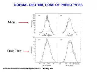
Normal Curves The study of normal curves can be traced back to the work ofthe great German mathematician Carl Friedrich Gauss, and forthis reason, normal curves are sometimes known as Gaussiancurves. Normal curves all share the same basic shape–that of abell–but otherwise they can differ widely in their appearance.
Normal Curves Some bells are short and squat,others are tall and skinny, andothers fall somewhere in between.
Normal Curves Mathematicallyspeaking,however, they all have the same underlying structure. In fact, whether a normal curve is skinny and tall or shortand squat depends on the choice of units on the axes, and anytwo normal curves can be made to look the same by just fiddling with the scales of the axes. What follows is a summary of some of the essential facts about normal curvesand their associated normal distributions.These facts are going to help us greatlylater on in the chapter.
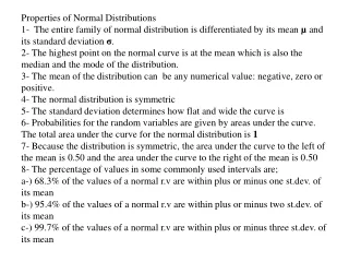
Essential Facts About Normal Curves Symmetry. Every normal curve has a vertical axis of symmetry, splitting the bell-shaped region outlined by the curve into two identicalhalves. This is the only line of symmetry of a normal curve, so we canrefer to it without ambiguity as the line of symmetry.
Essential Facts About Normal Curves Median / mean. We will call the point of intersection of the horizontalaxis and the line of symmetry of the curve the center of the distribution.
Essential Facts About Normal Curves Median / mean. The center represents both the medianM and themean (average) of the data. Thus, in a normal distribution, M = .The fact that in a normal distribution the median equals the mean implies that 50% of the data are less than or equal to the mean and 50%of the data are greater than or equal to the mean.
MEDIAN AND MEAN OF A NORMAL DISTRIBUTION In a normal distribution, M = . (If the distribution is approximately normal,then M ≈ .)
Essential Facts About Normal Curves Standard Deviation. The standard deviation–traditionally denoted by theGreek letter (sigma)–is an important measure of spread, and it is particularly useful when dealing with normal (or approximately normal) distributions, as we will see shortly. The easiest way to describe the standarddeviation of a normal distribution is to look at the normal curve.
Essential Facts About Normal Curves Standard Deviation. If you wereto bend a piece of wire into a bell-shaped normal curve, at the very top you would be bending the wire downward.
Essential Facts About Normal Curves Standard Deviation. But, at the bottom you would be bending the wire upward.
Essential Facts About Normal Curves Standard Deviation. As you move your handsdown the wire, the curvature gradually changes, and there is one point oneach side of the curve where the transition from being bent downward tobeing bent upward takes place. Such a point is called apoint of inflection of the curve.
Essential Facts About Normal Curves Standard Deviation. The standard deviation of a normal distribution is the horizontal distance between the line of symmetry of the curve and one of the two points of inflection, P´ or P in the figure.
STANDARD DEVIATION OF A NORMAL DISTRIBUTION In a normal distribution, the standard deviation equals the distance betweena point of inflection and the line of symmetry of the curve.
Essential Facts About Normal Curves Quartiles. We learned in Chapter 14 how to find the quartiles of a data set.When the data set has a normal distribution, the first and third quartilescan be approximated using the mean and the standard deviation . Themagic number to memorize is 0.675. Multiplying the standard deviation by0.675 tells us how far to go to the right or left of the mean to locate thequartiles.
QUARTILES OF A NORMAL DISTRIBUTION In a normal distribution, Q3 ≈ + (0.675) and Q1 ≈ – (0.675).
Example 16.3 A Mystery Normal Distribution Imagine you are told that a data set ofN = 1,494,531numbers has a normal distribution with mean = 515 and standard deviation = 114.For now, let’s notworry about the source of this data–we’ll discuss this soon. Just knowing the mean and standard deviation of this normal distributionwill allow us to draw a few useful conclusions about this data set.
Example 16.3 A Mystery Normal Distribution ■In a normal distribution, the median equals the mean, so the median value isM = 515.This implies that of the 1,494,531 numbers, there are 747,266 thatare smaller than or equal to 515 and 747,266 that are greater than or equal to 515.
Example 16.3 A Mystery Normal Distribution ■The first quartile is given byQ1≈ 515 – 0.675 114 ≈ 438.This impliesthat 25% of the data set (373,633 numbers) are smaller than or equal to 438. ■The third quartile is given byQ1≈ 515 + 0.675 114 ≈ 592.This impliesthat 25% of the data set (373,633 numbers) are bigger than or equal to 592.