Download
1 / 39
390 likes | 440 Views
Learn about the defining characteristics of normal distributions, including mean, standard deviation, symmetry, and probability calculations. Explore practical examples and applications in various scenarios.

E N D
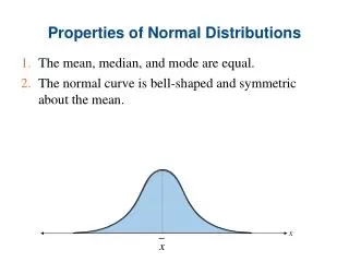
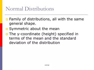
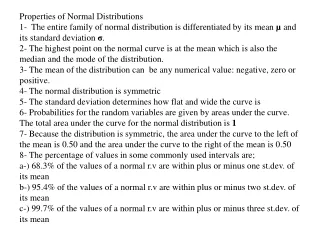
Properties of Normal Distributions 1- The entire family of normal distribution is differentiated by its mean µ and its standard deviation σ. 2- The highest point on the normal curve is at the mean which is also the median and the mode of the distribution. 3- The mean of the distribution can be any numerical value: negative, zero or positive. 4- The normal distribution is symmetric 5- The standard deviation determines how flat and wide the curve is 6- Probabilities for the random variables are given by areas under the curve. The total area under the curve for the normal distribution is 1 7- Because the distribution is symmetric, the area under the curve to the left of the mean is 0.50 and the area under the curve to the right of the mean is 0.50 8- The percentage of values in some commonly used intervals are; a-) 68.3% of the values of a normal r.v are within plus or minus one st.dev. of its mean b-) 95.4% of the values of a normal r.v are within plus or minus two st.dev. of its mean c-) 99.7% of the values of a normal r.v are within plus or minus three st.dev. of its mean
Find the area under the standard normal curve that lies 1- to the right of z = - 0.55 2- to the left of z = 0.84 3- to the right of z = 1.69 4- to the left of z = - 0.74 5- between z = 0.90 and z= 1.33 6- between z = -0.29 and z= 0.59
Q-1 - MOBILE PHONE Assume that the length of time, x, between charges of mobile phone is normally distributed with a mean of 10 hours and a standard deviation of 1.5 hours. Find the probability that the mobile phone will last between 8 and 12 hours between charges. Q-2 ALKALINITY LEVEL The alkalinity level of water specimens collected from the River in a country has a mean of 50 milligrams per liter and a standard deviation of 3.2 milligrams per liter. Assume the distribution of alkalinity levels is approximately normal and find the probability that a water specimen collected from the river has an alkalinity level A-) exceeding 45 milligrams per liter. B-) below 55 milligrams per liter. C-) between 51 and 52 milligrams per liter.
The grades of 400 students in a statistics course are normally distributed with mean µ = 65 and variance σ2=100 Q: Find the probability that a student selected randomly from this group would score within any interval given below. 1- A grade between 60 and 65 2- A grade between 70 and 65 3- A grade between 52 and 68 4- A grade that is greater than 85 5- A grade that is less than 72 6- A grade between 70 and 78
Example : 1 A normal distribution has the mean 74.4 Find its standard deviation if 10% of the area under the curve lies to the right of 100 Example : 2 A random variable has a normal distribution with standard deviation 10 . Find its mean if the probability is 0.8264 that it will take on a value less than 77.5 Example :3 For a certain random variable having the normal distribution, the probability is 0.33 that it will take on a value less than 245 and the probability is 0.48 that it will take on a value greater than 260. Find the mean and standard deviation of the random variable
Example Random samples of size n =2 are drawn from a finite population that consists of the numbers 2, 4, 6 and 8 without replacement. a-) Calculate the mean and the standard deviation of this population b-) List six possible random samples of size n=2 that can be drawn from this population and calculate their means. c-) Use the results in b-) to construct the sampling distribution of the mean. d-) Calculate the standard deviation of the sampling distribution.
Example for Correction Factor: What is the value of the finite population correction factor when a-) n= 20 and N=200 ? b-) n= 20 and N= 2000 ?
Example 2: Tuition Cost The mean tuition cost at state universities throughout the USA is 4,260 USD per year (2002 year figures). Use this value as the population mean and assume that the population standard deviation is 900 USD. Suppose that a random sample of 50 state universities will be selected. A-) Show the sampling distribution of x̄ (where x̄ is the sample mean tuition cost for the 50 state universities) B-) What is the probability that the random sample will provide a sample mean within 250 USD of the population mean? C-) What is the probability that the simple random sample will provide a sample mean within 100 USD of the population mean?
Example 1: A random variable of size 15 is taken from normal distribution with mean 60 and standard deviation 4. Find the probability that the mean of the sample is less than 58.
Example 5: Ping-Pong Balls The diameter of a brand of Ping-Pong balls is approximately normally distributed, with a mean of 1.30 inches and a standard deviation of 0.04 inch. If you select a random sample of 16 Ping-Pong balls, A-) What is the sampling distribution of the sample mean? B-) What is the probability that sample mean is less than 1.28 inches? C-) What is the probability that sample mean is between 1.31 and 1.33 inches? D-) The probability is 60% that sample mean will be between what two values, symmetrically distributed around the population mean?
Example 6: E-Mails Time spent using e-mail per session is normally distributed, with a mean of 8 minutes and a standard deviation of 2 minutes. If you select a random sample of 25 sessions, A-) What is the probability that sample mean is between 7.8 and 8.2 minutes? B-) What is the probability that sample mean is between 7.5 and 8.0 minutes? C-) If you select a random sample of 100 sessions, what is the probability that sample mean is between 7.8 and 8.2 minutes? D-) Explain the difference in the results of (A) and (C).
Types of Survey Errors • Coverage error • Non response error • Sampling error • Measurement error Excluded from frame Follow up on nonresponses Random differences from sample to sample Bad or leading question
Population Distribution Sampling Distribution Standard Normal Distribution ? ? ? ? ? ? ? ? ? ? Sample Standardize ? ? Z X
Sampling Distribution Properties As n increases, decreases Larger sample size Smaller sample size
Sampling Distribution Properties (i.e. is unbiased) Normal Population Distribution Normal Sampling Distribution (has the same mean) Variation:
How Large is Large Enough? • For most distributions, n ≥ 30 will give a sampling distribution that is nearly normal • For fairly symmetric distributions, n ≥ 15 • For normal population distributions, the sampling distribution of the mean is always normally distributed
Exercise - 1 A package-filling process at a Cement company fills bags of cement to an average weight of µ but µ changes from time to time. The standard deviation is σ = 3 pounds. A sample of 25 bags has been taken and their mean was found to be 150 pounds. Assume that the weights of the bags are normally distributed. Find the 90% confidence limits for µ.
Exercise - 3 An economist is interested in studying the incomes of consumers in a particular region. The population standard deviation is known to be $1,000. A random sample of 50 individuals resulted in an average income of $15,000. What is the upper end point in a 99% confidence interval for the average income?
Exercise - 4 An economist is interested in studying the incomes of consumers in a particular region. The population standard deviation is known to be $1,000. A random sample of 50 individuals resulted in an average income of $15,000. What is the width of the 90% confidence interval?
Exercise - 5 The head librarian at the Library of Congress has asked her assistant for an interval estimate of the mean number of books checked out each day. The assistant provides the following interval estimate: from 740 to 920 books per day. If the head librarian knows that the population standard deviation is 150 books checked out per day, and she asked her assistant for a 95% confidence interval, approximately how large a sample did her assistant use to determine the interval estimate?
STEP BY STEP Critical Value Approach to Hypothesis Testing 1- State Ho and H1 2- Choose level of significance, α Choose the sample size, n 3- Determine the appropriate test statistics and sampling distribution. 4- Determine the critical values that divide the rejection and non-rejection areas. 5- Collect the sample data, organize the results and compute the value of the test statistics. 6- Make the statistical decision and state the managerial conclusion If the test statistics falls into non-rejection region, DO NOT REJECT Ho If the test statistics falls into rejection region, REJECT Ho The managerial conclusion is written in the context of the real world problem.
Exercise –Hourly wage The president of a company states that the average hourly wage of his/her employees is 8.65 TRL. A sample of 50 employees has the distribution shown below. At α=0.05, is the president’s statement believable? Assume σ=0.105 TRL M fM fM2 _______ 8.39 16.78 140.7842 8.48 50.88 431.4624 8.57 102.84 881.3388 8.66 155.88 1349.9208 8.75 87.5 765.625 8.84 17.68 156.2912 431.56 3725.4224 Class Freq. 8.35-8.43 2 8.44-8.52 6 8.53-8.61 12 8.62-8.70 18 8.71-8.79 10 8.80-8.88 2 Total: 50
Exercise – Athletic Shoes A researcher claims that the average cost of men`s athletic shoes is less than 80 USD. He selects a random sample of 36 pairs of shoes from a catalog and finds the following costs. Is there enough evidence to support the researcher`s claim at α = 0.10. Assume σ=19.2 ∑x =2700
Exercise – Life Guards A researcher wishes to test the claim that the average age of lifeguards in a city is greater than 24 years. She selects a sample of 36 guards and finds the mean of the sample to be 24.7 years with a standard deviation of 2 years. Is there evidence to support the claim at α = 0.05? Use p-value method.
Exercise – Assist. Prof. A researcher reports that the average salary of assistant professors is more than 42,000 TL. A sample of 30 assistant professors has a mean salary of 43,260 TL. At α = 0.05, Test the claim that assistant professors earn more than 42,000 TL a year. The population standard deviation is 5,230 TL.
Exercise – Wind Speed A researcher claims that the average wind speed in a certain city 8 miles per hour. A sample of 32 days has an average wind speed of 8.2 miles per hour. The standard deviation of the sample is 0.6 mile per hour. At α = 0.05, is there enough evidence to reject the claim? Use p-value method.
Exercise – Sugar Sugar is packed in 5 kg bags. An inspector suspects the bags may not contain 5 kg. A sample of 50 bags produces a mean of 4.6 kg and a standard deviation of 0.7 kg. Is there enough evidence to conclude that the bags do not contain 5 kg as stated at α = 0.05? Also find the 95% CI of the true mean.
ACTUAL SITUATION STATISTICAL DECISION H0IS FALSE H0IS TRUE DO NOT REJECT H0 REJECT H0 If the null hypothesis is true and accepted or false and rejected the decision is in either case CORRECT. If the null hypothesis is true and rejected or false and accepted the decision is in either case in ERROR.
Exercise – 3 The manager of the women`s dress department of a department store wants to know whether the true average number of women`s dresses sold per day is 24. If in a random sample of 36 days the average number of dresses sold is 23 with a standard deviation of 7 dresses, Is there, at the 0.05 level of significance, sufficient evidence to reject the null hypothesis that µ=24?