Download
1 / 35
350 likes | 484 Views
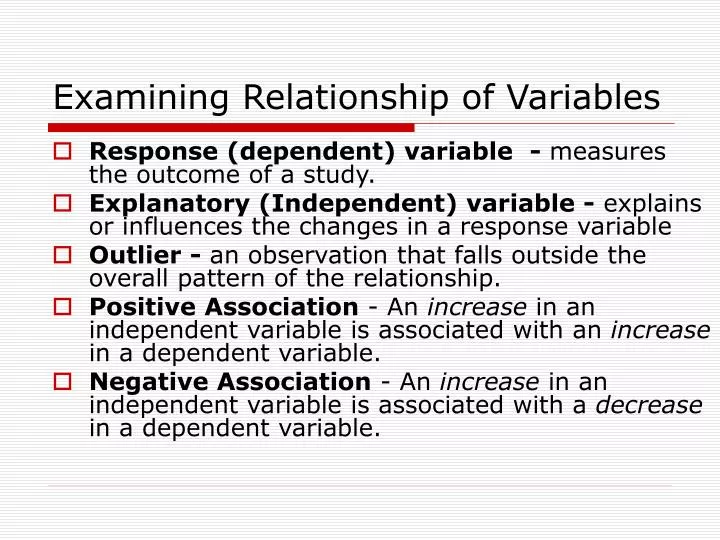
Examining Relationship of Variables. Response (dependent) variable - measures the outcome of a study. Explanatory (Independent) variable - explains or influences the changes in a response variable Outlier - an observation that falls outside the overall pattern of the relationship.

E N D
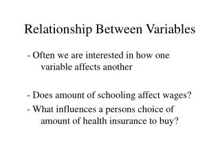
Examining Relationship of Variables • Response (dependent) variable - measures the outcome of a study. • Explanatory (Independent) variable - explains or influences the changes in a response variable • Outlier - an observation that falls outside the overall pattern of the relationship. • Positive Association - An increase in an independent variable is associated with an increase in a dependent variable. • Negative Association - An increase in an independent variable is associated with a decrease in a dependent variable.
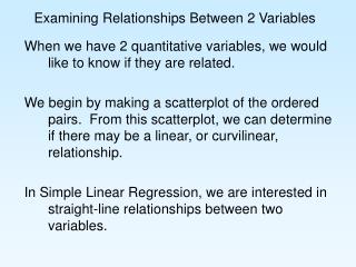
Scatterplot • Shows relationship between two variables (age and height in this case). • Reveals form, direction, and strength of the relationship.
Scatterplot - Demo • MS-Excel: • Step 1: Select Chart wizard • Step 2: From the chart type select XY(Scatter) • Step 3: Select Chart from chart sub type and click next • Step 4: Data range: range for variable in the x axis (age in our case), range for the variable in the y axis (hgt in our case) and click on next • Step 5: Click on titles to write title and labels of the chart , click on axes and mark on Value (X) and Value (Y) axis , click on Gridlines and take all the mark off( if you want no gridlines), click on legend and put options of legend (if you don’t want legend) then click on Finish
Scatterplot - Demo • SPSS: • Step 1: Click on Graphs and select Scatter/Dot • Step 2: Select Simple scatter • Step 3: Select variables for Yaxis (usually response variable) and Xaxis (explanatory variable) and click on Titles to write titles in Line 1. After writing title click on ‘Continue’. • Step 4: Click on ‘Ok’. • R: • plot(x, y, main= “Title name”, xlab=“x axis label name”, ylab=“y axis label name” ) where x and y are the data of two variables and for our example x is age and y is hgt.
Scatterplots Strong positive association Strong negative association Points are scattered with a poor association
Correlation of two variables • Correlation measures the direction and strength of the relationship between two quantitative variables. Suppose that we have data on variables x and y for n individuals. Then the correlation coefficient r between x and y is defined as, Where, sx and sy are the standard deviations of x and y. • r is always a number between -1 and 1. Values of r near 0 indicate little or no linear relationship. Values of r near -1 or 1 indicate a very strong linear relationship. • The extreme values r=1 or r=-1 occur only in the case of a perfect linear relationship, when the points lie exactly along a straight line.
Correlation of two variables • Positive r indicates positive association i.e. association between two variables in the same direction, and negative r indicates negative association. • Scatterplot of Height and Age shows that these two variables possess a strong, positive linear relationship. The correlation coefficient of these two variables is 0.9829632, which is very close to 1.
Correlation of two variables r=0.98 r=-0.96 r=0.02
Correlation of two variables • MS-Excel: • Step 1: Click on function Wizard fx • Step 2: Select function Correl • Step 3: Input range Array 1 and Array 2 (for our example age and hgt) and click on Ok. • Another option: • Check if the data of two variables are in a side by side position. If not, copy and paste them side by side in a new worksheet and follow the following steps- • Step 1: Select Data Analysis from the menu Tools • Step 2: Select Correlation and type or select Input and Output range and click on ok.
Correlation of two variables • SPSS: • Step 1: Select Correlate from the menu Analyze • Step2: Click on Bivariate and select the variables (age and hgt) and click on Ok • R: cor( variable 1, variable 2) e.g. age and hgt are the variable 1 and variable 2 in our example
Example 1: Calculating Correlation Coefficient of the variables Height and Age in our data set. • MS-Excel: Click on function Wizard fx > Correl > Input range Array 1: age Input range Array 1: hgt > ok. It gives correlation coefficient, r=.98. or Tools > data analysis > correlation > range for variables age and hgt > ok. It gives you the following results.
Example 1: Calculating Correlation Coefficient of the variables Height and Age in our data set. • SPSS: Analyze > Correlate > Bivariate > select age and hgt > ok. It gives the following result
Example 1: Calculating Correlation Coefficient of the variables Height and Age in our data set. • R: >cor(age, hgt). It gives the correlation coefficient 0.98296
Strong Association but no Correlation Gas mileage of an auto mobile first increases than decreases as the speed increases like the following data: Scatter plot shows an strong association. But calculated, r = 0, why? r = 0 ? It’s because the relationship is not linear and r measures the linear relationship between two variables.
Influence of an outlier • Consider the following data set of two variables X and Y: r = -0.237 • After dropping the last pair, r = 0.996
Simple Linear Regression • Regression refers to the value of a response variable as a function of the value of an explanatory variable. • A regression model is a function that describes the relationship between response and explanatory variables. • A simple linear regression has one explanatory variable and the regression line is straight. • The linear relationship of variable Y and X can be written as in the following regression model form Y= b0 + b1X + e where, ‘Y’ is the response variable, ‘X’ is the explanatory variable, ‘e’ is the residual (error), and b0 and b1 are two parameters. Basically, bo is the intercept and b1 is the slope of a straight line y= b0 + b1X.
Simple Linear Regression A simple regression line is fitted for height on age. The intercept is 31.019 and the slope (regression coefficient) is .1877.
Simple Linear RegressionAssumptions: • Response variable is normally distributed. • Relationship between the two variables is linear. • Observations of response variable are independent. • Residual error is normally distributed with mean 0 and constant standard deviation.
Simple Linear Regression • Estimating Parameters b0 and b1 • Least Square method estimates b0 and b1 by fitting a straight line through the data points so that it minimizes the sum of square of the deviation from each data point. • Formula:
Simple Linear Regression • Fitted Least Square Regression line • Fitted Line: • Where is the fitted / predicted value of ith observation (Yi) of the response variable. • Estimated Residual: • Least square method estimates b0 and b1 to minimize the summed error:
Simple Linear Regression • Fitted Least Square Regression line In this example, a regression line (red line) has been fitted to a series of observations (blue diamonds) and residuals are shown for a few observations (arrows). e3 e1 e2
Simple Linear Regression • Interpretation of the Regression Coefficient and Intercept • Regression coefficient (b1) reflects the change in the response variable Y for a unit change in the explanatory variable X. That is, the slope of the regression line. • Intercept (b0) estimates the value of the response variable Y without the influence of the explanatory variable X. That is, when the explanatory variable = 0.0.
Simple Linear Regression • MS-Excel: • Step1: Select Data Analysis from the menu Tools • Step2: Input Y range: range for the response (dependent) variable, Input X range: range for the independent variable • Step 3: Make selections of out puts you want and click on ok • SPSS: • Step 1: Select Regression from the menu Analyze • Step 2: Select Linear and then for Dependent: Select dependent variable and for Independent(s): select Independent variable • Step 3: Click on Statistics and select options, clik on Plots and select variables for scatter plots (if you want), click on continue an d then ok • R: lm(y~x, data) summary(lm(y~x, data)) where, y is the dependent variable, x is the independent variable and data is a data frame containing the variables in the model.
Example 2: R Linear Regression output: Height on age >lm (hgt ~ age) gives the following output Call: lm(formula = hgt ~ age) Coefficients: (Intercept) age 31.0187 0.1877 R code summary (lm (hgt ~ age) ) gives the following output Call: lm(formula = hgt ~ age) Residuals: Min 1Q Median 3Q Max -2.53975 -0.55722 0.08105 0.68147 2.24326 Coefficients: Estimate Std. Error t value Pr(>|t|) (Intercept) 31.018720 0.439077 70.64 <2e-16 *** age 0.187735 0.004609 40.73 <2e-16 *** --- Signif. codes: 0 ‘***’ 0.001 ‘**’ 0.01 ‘*’ 0.05 ‘.’ 0.1 ‘ ’ 1 Residual standard error: 1.07 on 58 degrees of freedom Multiple R-Squared: 0.9662, Adjusted R-squared: 0.9656 F-statistic: 1659 on 1 and 58 DF, p-value: < 2.2e-16
Multiple Regression • Two or more independent variables to predict a single dependent variable. • Multiple regression model of Y on p number of explanatory variables can be written as, Y = b0 + b1X1 + b2X2 +… +bpXp +e where bi (i=1,2, …, p) is the regression coefficient of Xi
Multiple Regression • Fitted Y is given by, • The estimated residual error is the same as that in the simple linear regression,
Multiple Regression • MS-Excel: Every thing is the same as for the simple regression except we need to select multiple columns for the range of independent variables. If the columns of independent variables are not side by side, then we need to have them side by side. For that we can insert another excel sheet and copy the data from original sheet and paste the data in the new sheet. We first copy the dependent variable and paste that in one of the columns and then copy independent variables and paste them in side by side columns. • SPSS: Everything is the same as for the simple regression except we select more than one independent variables. • R: Every thing is the same as for the simple regression except adding more independent variables in the model. i.e. lm(y~x1 + x2 , data) summary(lm(y~x1 + x2 , data)) where, y is the dependent variable, x1 and x2 are independent variables and data is a data frame containing the variables in the model.
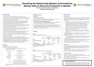
Example 3: MS Excel Multiple Regression output: Height on Age and PLUC.post
Example 3: SPSS Multiple Regression output: Height on Age and PLUC.post
Example 3: R Multiple Regression output: Height on Age and PLUC.post R code lm(hgt ~ age + PLUC.post) gives the following output Coefficients: (Intercept) age PLUC.post 31.3297 0.1880 -0.0279 R code summary(lm(hgt~age+PLUC.post)) gives the following output Residuals: Min 1Q Median 3Q Max -2.52512 -0.57195 0.02261 0.74912 2.21156 Coefficients: Estimate Std. Error t value Pr(>|t|) (Intercept) 31.329680 0.752489 41.635 <2e-16 *** age 0.188043 0.004678 40.196 <2e-16 *** PLUC.post -0.027899 0.054644 -0.511 0.612 --- Signif. codes: 0 ‘***’ 0.001 ‘**’ 0.01 ‘*’ 0.05 ‘.’ 0.1 ‘ ’ 1 Residual standard error: 1.077 on 57 degrees of freedom Multiple R-Squared: 0.9664, Adjusted R-squared: 0.9652 F-statistic: 819 on 2 and 57 DF, p-value: < 2.2e-16
Coefficient of Determination (Multiple R-squared) • Total variation in the response variable Y is due to (i) regression of all variables in the model (ii) residual (error). • Total variation of y, SS (y) = SS(Regression) +SS(Residual) • The Coefficient of Determination is,
Coefficient of Determination (Multiple R-squared) • R2 lies between 0 and 1. • R2 = 0.8 implies that 80% of the total variation in the response variable Y is due to the contribution of all explanatory variables in the model. That is, the fitted regression model explains 80% of the variance in the response variable.
Example 4: Calculating coefficient of determination for the variables in example 3. • MS-Excel: It’s in the MS-Excel output of Example 3. • SPSS: It’s in the SPSS output of Example 3. • R: It’s in the R output of Example 3.