Relationship Between Variables
Relationship Between Variables. - Often we are interested in how one variable affects another - Does amount of schooling affect wages? - What influences a persons choice of amount of health insurance to buy?. Correlation Coefficient

Relationship Between Variables
E N D
Presentation Transcript
Relationship Between Variables - Often we are interested in how one variable affects another - Does amount of schooling affect wages? - What influences a persons choice of amount of health insurance to buy?
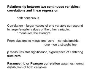
Correlation Coefficient Sometimes, we wish to obtain the indicator of the strength of the linear relationship between two variables y and x that is independent of their respective scales of measurements. This indicator of strength of the linear relationship between two variables is called correlation coefficient r. r is a standardized measure of a bivariate linear relationship between two variables x and y. (r) Is a a way to measure how “scattered” a relationship is
Using STATA twoway scatter value homeruns
Correlation coefficient Sample standard deviation of x Sample standard deviation of Y Covariance of x and y
Implications of r: *Negative value of r: high values of Y tend to occur with low values of X and low Y with high X *Positive value of r:high values of Y tend to occur with high values of X, and low Y with low X . correlate value homeruns | value homeruns -------------+------------------ value | 1.0000 homeruns | 0.6667 1.0000
corr value caught_stealing • | value caught~g • -------------+------------------ • value | 1.0000 • caught_ste~g | 0.3554 1.0000 Note how the graphs looked and the difference in correlation.
Econometrics Welcome to what we economists like to call our own Estimating the relationship between variables
* Assume that we are dealing with a single relationship and that it contains only two variables: Y= f (x) value= f (homeruns) * Choose the function form of the relationship between Y and X: (linear equation) Some other possibilities are: which implies which implies These two forms, which are nonlinear can be transformed by taking natural logs of both sides. Then the resulting logged equations are linear in the logs
Why a stochastic error term: • Over and above the total effect of all relevant factors, there is a basic and unpredictable element of randomness which can be adequately characterized only buy the inclusion of a random error term.
: intercept : slope
Assumptions about the stochastic model: • i=1,2,3…… • for all i • if i ~= j • if i=j • - It is also nice is the error term is normally distributed
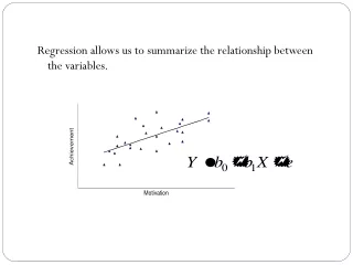
Goal of regression: find the relationship between Y and X, causality, or predict effects The relationship is determined by the coefficients of the equation. So the problem is: given data of Y and X, how to estimate the and This problem can also expressed this way: how to choose a line which can fit the data scatter best. One standard way is to choose a line which will minimize the difference between the actual Y and estimated Y , or in other words minimize the estimation error
Why might there be estimation errors? • There is information we don’t have that would allow us to completely explain the variation in Y. • There are random errors of observation, measurement, sampling, or all of the above. • The same reason the population relationship has an error
Denote the estimated line through the data as: =estimates of two unknown parameters =estimated value of Y for X =the difference between the actual an estimated values of Y Consequently, the our goal is to minimize: This approach is called least squares estimation
Are Least Square estimate parameters good estimate or not? • If the assumptions about the error term hold, then • least squares estimators of the slope and intercept terms are unbiased estimators. • Least squares estimators of the slope and intercept terms are most efficient linear estimators. They are the best linear unbiased estimator (BLUE), which means among all the linear and unbiased estimators, least square estimators’ variance is smallest
Are random variables? • Are random variables? • For the estimates to be unbiased • It can be shown that are the most efficient.
We can also find the standard error of the estimates • There are many ways to represent this but the following way uses information we already know • The standard error for the intercept term can also be found but will not be presented in this class.
How to do these by using STATA • . regress value homeruns • Source | SS df MS Number of obs = 334 • -------------+------------------------------ F( 1, 332) = 265.63 • Model | 12074.6163 1 12074.6163 Prob > F = 0.0000 • Residual | 15091.2999 332 45.4557225 R-squared = 0.4445 • -------------+------------------------------ Adj R-squared = 0.4428 • Total | 27165.9162 333 81.5793278 Root MSE = 6.7421 • ------------------------------------------------------------------------------ • value | Coef. Std. Err. t P>|t| [95% Conf. Interval] • -------------+---------------------------------------------------------------- • homeruns | .5788295 .0355147 16.30 0.000 .5089673 .6486918 • _cons | 3.387263 .6229686 5.44 0.000 2.1618 4.612726 • ------------------------------------------------------------------------------
Interpretation: A player’s value increases by 0.5788 for each homerun. Each additional homerun adds 0.5788 to the players value
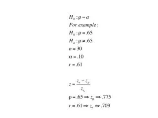
Testing the relationship between x and y If there were no relationship between x and y what would you expect to be? If the error term is normally, identically and independently distributed, we can form the t- statistic, which follows z/t-distribution with d.f.=n-K:
Hypothesis test • hypothesis: • Test statistic: • Critical value (d.f = n-K): • 4) You could also use the p-value!
Based on the sampling distribution of estimate coefficients, we can also confidence intervals. Confidence Intervals: With d.f.=n-K
regress value homeruns • Source | SS df MS Number of obs = 334 • -------------+------------------------------ F( 1, 332) = 265.63 • Model | 12074.6163 1 12074.6163 Prob > F = 0.0000 • Residual | 15091.2999 332 45.4557225 R-squared = 0.4445 • -------------+------------------------------ Adj R-squared = 0.4428 • Total | 27165.9162 333 81.5793278 Root MSE = 6.7421 • ------------------------------------------------------------------------------ • value | Coef. Std. Err. t P>|t| [95% Conf. Interval] • -------------+---------------------------------------------------------------- • homeruns | .5788295 .0355147 16.30 0.000 .5089673 .6486918 • _cons | 3.387263 .6229686 5.44 0.000 2.1618 4.612726 • ------------------------------------------------------------------------------
. regress value age • Source | SS df MS Number of obs = 334 • -------------+------------------------------ F( 1, 332) = 3.48 • Model | 281.561913 1 281.561913 Prob > F = 0.0631 • Residual | 26884.3543 332 80.9769706 R-squared = 0.0104 • -------------+------------------------------ Adj R-squared = 0.0074 • Total | 27165.9162 333 81.5793278 Root MSE = 8.9987 • ------------------------------------------------------------------------------ • value | Coef. Std. Err. t P>|t| [95% Conf. Interval] • -------------+---------------------------------------------------------------- • age | -.2210561 .1185486 -1.86 0.063 -.4542571 .0121449 • _cons | 18.16414 3.571044 5.09 0.000 11.13942 25.18887 • ------------------------------------------------------------------------------
Prediction *Is estimate of Y a random variable? *What distribution does the estimate of Y have?. follows t-distribution with d.f.=n-K the mean is and standard deviation is
Point estimate: • Confidence interval estimate:
Example: Using the regression of value on homeruns what would be the predicted value of a player who hits 30 homeruns a season?
Using STATA to do prediction . predict hrhat (computes predicted values of Y) . predict SEhrhat, stdp (compute )
Overall Goodness-of-fit How well does the estimated regression line fit the observations? In other words, how much the the line explain the variation of dependent variable? Note: This question is different from are the estimates significant or not? The perfect regression line should includes all data points with no error. 100% of the variation of Y is explained by X
*Total sum of squares (TSS) is the sum of squared deviations of the dependent variable around its mean and is a measure of the total variability of the variable: *Explained sum of squares (ESS) is the sum of squared deviations of predicted values of Y around its mean: *Residual sum of squares (RSS) is the sum of squared deviations of the residuals around their mean value of zero:
*Decomposition of variation of Y: * The measure of goodness-of-fit is the proportion the variation of Y that is explained by the model. This measure is called R2 * Property of R2: 1) 2) The closer R2 is to 1, the better model fits the data.
regress value homeruns • Source | SS df MS Number of obs = 334 • -------------+------------------------------ F( 1, 332) = 265.63 • Model | 12074.6163 1 12074.6163 Prob > F = 0.0000 • Residual | 15091.2999 332 45.4557225 R-squared = 0.4445 • -------------+------------------------------ Adj R-squared = 0.4428 • Total | 27165.9162 333 81.5793278 Root MSE = 6.7421 • ------------------------------------------------------------------------------ • value | Coef. Std. Err. t P>|t| [95% Conf. Interval] • -------------+---------------------------------------------------------------- • homeruns | .5788295 .0355147 16.30 0.000 .5089673 .6486918 • _cons | 3.387263 .6229686 5.44 0.000 2.1618 4.612726 • ------------------------------------------------------------------------------
What type of variable can be included in regression? • Of course any continuous variable can be included. • It is permissible to represent these as discrete variable, like an interval, interpretation does not change • Example • Age, income, years of education, ect.
What type of variable can be included in regression? • Dummy variables • These are variable that take on one value or another. One realization is assigned the value of one and the other the value of 0. • Example • If male – Gender = 1, if Female – Gender = 0 • Interpretation: The average value of the dependent variable for all people with a value of 1 on the dummy variable minus the average value of the dependent variable for all people with 0 on the dummy variable.
Example: Affairs Dataset kids = 1 if individual has kids, 0 otherwise • Source | SS df MS Number of obs = 601 • -------------+------------------------------ F( 1, 599) = 6.55 • Model | 70.632204 1 70.632204 Prob > F = 0.0107 • Residual | 6458.44933 599 10.7820523 R-squared = 0.0108 • -------------+------------------------------ Adj R-squared = 0.0092 • Total | 6529.08153 600 10.8818026 Root MSE = 3.2836 • ------------------------------------------------------------------------------ • affairs | Coef. Std. Err. t P>|t| [95% Conf. Interval] • -------------+---------------------------------------------------------------- • kids | .7598123 .2968627 2.56 0.011 .1767941 1.342831 • _cons | .9122807 .2511034 3.63 0.000 .4191306 1.405431 • ------------------------------------------------------------------------------
What type of variable can be included in regression? • Ordinal variables – The numbers tell you the order but do not tell you the magnitude of difference between one value and another. • It is not technically proper to use ordinal variables but we have to because of lack of better information. • Interpretation: best to look at direction and significance. If a person is more of the independent variable they will be more/less likely the dependent variable
Example: Affairs Dataset marriage_rating = rating scale from 5 best to 1 worst • Source | SS df MS Number of obs = 601 • -------------+------------------------------ F( 1, 599) = 50.76 • Model | 510.098751 1 510.098751 Prob > F = 0.0000 • Residual | 6018.98278 599 10.0483853 R-squared = 0.0781 • -------------+------------------------------ Adj R-squared = 0.0766 • Total | 6529.08153 600 10.8818026 Root MSE = 3.1699 • ---------- -------------------------------------------------------------------- • affairs | Coef. Std. Err. t P>|t| [95% Conf. Interval] • -------------+---------------------------------------------------------------- • marriage_r~g | -.8358057 .1173076 -7.12 0.000 -1.06619 -.6054214 • _cons | 4.742111 .4790101 9.90 0.000 3.801368 5.682854 • ------------------------------------------------------------------------------