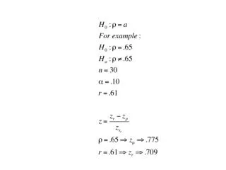
Download
1 / 45
450 likes | 556 Views
Mathematical description of the relationship between two variables using regression. Lecture 13 BIOL2608 Biometrics. Regression Analysis. A simple mathematical expression to provide an estimate of one variable from another

E N D
Mathematical description of the relationship between two variables using regression Lecture 13 BIOL2608 Biometrics
Regression Analysis • A simple mathematical expression to provide an estimate of one variable from another • It is possible to predict the likely outcome of events given sufficient quantitative knowledge of the processes involved
Regression models y x • Model 1 • “Controlled” parameter (Independent variable) vs. Measured parameter (dependent variable) • Independent variable (on x-axis) must be measured with a high degree of accuracy & is not subjected to random variation • Other inferential factors must be kept constant • Dependent variable (on y-axis) may vary randomly and its ‘error’ should follow a normal distribution
Normally distributed populations of y values Y X • The population of y values is normally distributed & • The variances of different population of y values corresponding to different individual x values are similar
Regression models x2 x1 • Model 2 • Both measured parameters (x1 & x2 not x & y) which cannot be controlled • Both are subject to random variation & called random-effects factors • Common in field studies where conditions are difficult to control • Correlation rather than regression, required for bivariately normal distributions • e.g. measurements of human arm and leg lengths
Example for model 1 • Study the rate of disappearance of a pesticide in a seawater sample • Time (independent) vs. Concentration (dependent) • Other factors such as pH, salinity must be kept constant • Study the growth rate of fish at different fixed water temperature • Temp (independent) vs. Growth rate (dependent) • Other factors such as diet, feeding frequency must be kept constant
Y x, y c d a X Model: y = a + bx Slope: coefficient b = c/d Intercept: coefficient a
b= -ve b= +ve Y b= 0 X
The concept of least squares Sum of di2 indicates the deviations of the points from the regression line Best fit line is achieved with minimum sum of square deviations (di2) d
Calculation for a regression • y = a + bx • b = [xy – (xy/n)]/ [x2 – (x)2/n] • a = y – bx b = [514.8-(130)(44.4)/13]/[1562 – (130)2/13] b = 0.720 cm/day a = 3.4 – (0.720)(10) = 0.715 cm The simple linear regression equation is Y = 0.715 + 0.270X ^
Normally distributed populations of y values Y X • The population of y values is normally distributed & • The variancesof different population of y values corresponding to different individual x values are similar
^ Residual = y – y = y – (a + bx) + + 0 0 - - + + 0 0 - -
Testing the significance of a regression Source of variation Sum of squares (SS) DF Mean square (MS) Total (Yi- Y) Yi2 – (Yi)2/n n –1 Linear regression [XiYi - XiYi/n]2 1 regression SS (Yi – Y) Xi2 – (Xi)2/n regression DF Residual (Yi – Yi) total SS – regression SS n – 2 residual SS residual DF ^ ^ Compute F = regression MS/ residual MS, the critical F(1), 1, (n-2) Coefficient of determination r2 = regression SS/total SS r2 indicates the proportion (or %) of the total variation in Y that is explained or accounted by fitted the regression: e.g. r2 = 0.81 i.e. the regression can explain 81% of the total variation
ANOVA testing of Ho: b = 0 Total SS = 171.3 – (44.4)2/13 = 19.66 Regression SS = [514.8-(130)(44.4)/13]2/[1562 – (130)2/13] = 19.13 Residual SS = 19.66 – 19 .13 = 0.53 Total DF = n –1 = 12 Source of variation SS DF MS F Crit F P Total 19.66 12 Linear regression 19.13 1 19.13 401.1 4.84 <0.001 Residual 0.53 11 0.048 Thus, reject Ho. r2 = 19.13/19.66 = 0.97 =(Sy·x)2
How to report the results in texts? Source of variation SS DF MS F Crit F P Total 19.66 12 Linear regression 19.13 1 19.13 401.1 4.84 <0.001 Residual 0.53 11 0.048 Thus, reject Ho. r2 = 19.13/19.66 = 0.97 The wing length of the sparrow significantly increases with increasing age (F1, 11 = 401.1, r2 = 0.97, p < 0.001). 97% of the total variance in the wing length data can be explained by age.
Confidence intervals of the regression coefficients • Assume that the slopes b of a regression are normally distributed, then it is possible to fit confidence intervals (CI) to the slope: • 95% CI = b t (2), (n-2) Sb where Sb = (Sy·x)2/( Xi2 – (Xi)2/n) • CI for the interceptYi = Yi t (2), (n-2) SYi where SYi = (Sy·x)2[1/n + (Xi – X)2/( Xi2 – (Xi)2/n)]
Standard errors of predicted values of Y(follow the same example) ^ Y = 0.715 + 0.270X, mean = 10 If x = 13 days, then y = 4.225 cm • SYi = (Sy·x)2[1/n + (Xi – X)2/( Xi2 – (Xi)2/n)] = (0.0477)[1/13 + (13 –10)2/(1562 – 1302/13)] = 0.073 cm • CI for the intercept Yi = Yi t 0.05(2), 11 SYi = 4.225 (2.201)(0.073) = 4.225 0.161 cm
Inverse prediction (follow the same example) ^ Y = 0.715 + 0.270X and mean Y = 3.415, if Yi = 4.5, then X = (Yi – 0.715)/0.270 = 14.019 days To compute 95% CI: t 0.05(2), 11 = 2.201 K = b2 –t2Sb2 = 0.2702 – (2.201)2[(Sy·x)2/( Xi2 – (Xi)2/n)] = 0.2702 – (2.201)2[(0.0477)/(262)] = 0.0720 95% CI: =X + b(Yi – Y)/K (t/K)(Sy·x)2{[(Yi – Y)2/( Xi2 – (Xi)2/n)]+K(1 + 1/n)} =14.069 (0.270/0.072) (0.0477){[(4.5 – 3.415)2/262]+ 0.072(1 + 1/13)} = 14.069 1.912 days Lower limit = 12.157 days; Higher limit = 15.981 Important for toxicity test
Regression with replication See p. 345 – 357, example 17.8 (Zar, 1999)
Example 17.8 Total SS (DF = 20 –1) = 383346 – (2744)2/20 = 6869.2 Regression SS (DF = 1) = [149240-(1050)(2744)/20]2/[59100 – (1050)2/20] = (5180)2/3975 = 6751.29 Among-groups SS (DF = k –1 = 5 – 1 = 4) = 383228.73 – (2744)2/20 = 6751.93 Within groups SS (DF = total – among-groups = 19 – 4 = 15) = 6869.2 – 6751.93 = 117.27 Deviations-from-linearity SS (DF = among-groups – regression = 4 –1 = 3) = 6751.93 – 6751.29 = 1.64 b = [149240-(1050)(2744)/20]/ [59100 – (1050)2/20] = 5180/3975 = 1.303 mm Hg/yr Mean x = 52.5; mean y = 137.2 a = 137.2 – (1.303)(52.5) = 68.79 mm Hg Y = 68.79 + 1.303x
Ho: The population regression is linear. Source of variation SS DF MS F P Total 6869.2 19 Among groups 6751.93 4 Linear regression 6750.29 1 Deviations from linearity 1.64 3 0.55 0.07 >0.25 Within groups 117.27 15 7.82 Thus, accept Ho. Ho: = 0 Source of variation SS DF MS F P Total 6869.2 19 Linear regression 6750.29 1 6750.29 1021.2 <0.001 Within groups 118.91 18 6.61 Thus, reject Ho. r2 = 6750.29/6869.2 = 0.98
Model 2 regression • The regression coefficient b’ (b prime) is obtained as Sx1/Sx2 • e.g. field observations of PCB (polychlorinated biphenyl) concentration per gram of fish and compared with the kidney biomass
b’ = 1.2074/2.2033 = -0.548 (by inspection of the scatter-graph) a’ = mean X1 – b(mean X2) = 9.739 – 0.548(5.835) = 12.94 X1 = 12.94 – 0.548X2
Key notes • There are two regression models • Model 1 regression is used when one of the variable is fixed so that it is measured with negligible error • In model 1, the fixed variable is called the independent variable x and the dependent variable is designated y. • The regression equation is written y = a + bx where a and b are the regression coefficients • Model 2 regression is used where neither variable is fixed and both are measured with error.
Comparing simple linear regression equations &Multiple regression analysis
Comparing Two Slopes • Use of Student’s t t = (b1 – b2) / Sb1-b2 Sb1-b2 = (SY·X)p2/(x2)1 + (SY·X)p2/(x2)2 Y Y Y X X X
Comparing Two Slopes • (SY·X)p2= (residual SS)1 + (residual SS)2 • (residual DF)1 + (residual DF)2 • Critical t : DF = n1 + n2 – 4 • Test Ho: Equal slopes Y Y Y X X X
b = 2.97 Y Comparing Two Slopes - Example x2 = Xi2 – ( Xi)2/n xy= XiYi – ( XiYi/n) y2 = Yi2 – ( Yi)2/n b = 2.17 X • For sample 1: Temperature (C) For sample 2: Volumes (ml) • x2 = 1470.8712 x2 = 2272.4750 • xy=4363.1627 xy= 4928.8100 • y2 =13299.5296 y2 =10964.0947 n = 26 n = 30 b = xy/ x2 b = 4363.1627/1470.8712 = 2.97 b = 4928.8100/2272.4750 = 2.17 Residual SS = RSS = y2 –( xy)2/ x2 = 13299.5296 – (4363.1627)2/1470.8712 = 10964.0947 – (4928.81)2/2272.475 = 356.7317 = 273.9142 Residual DF = RDF = n –2 = 26 – 2 = 30 - 2 = 28 (SY·X)p2 = (RSS1 + RSS2)/(RDF1 + RDF2) = (356.7317+ 273.9142)/(24+28) = 12.1278
(SY·X)p2 = (RSS1 + RSS2)/(RDF1 + RDF2) = (356.7317+ 273.9142)/(24+28) = 12.1278 Sb1-b2 = (SY·X)p2/(x2)1 + (SY·X)p2/(x2)2 = (12.1278)/(1470.8712) + (12.1278)/(2272.4750) = 0.1165 t = (2.97 – 2.17) / 0.1165 = 6.867 (p < 0.001) DF = 24 + 28 = 52, Critical t 0.05(2), 52 = 2.007 Reject Ho. Therefore, there is a significant difference between the two slopes (t 0.05(2), 52 = 6.867, p < 0.001) b = 2.97 Y b = 2.17 X
b = 2.97 Y Testing for difference between points on the two nonparallel regression lines. We are testing whether the volumes (Y) are different in the two groups at X = 12: Ho: same value Further we need to know A1 = 10.57 and a2 = 24.91; Mean X1 = 22.93 and mean X2 = 18.95 Then, Y = a + bX Estimated Y1 = 46.21; Y2 = 50.95 SY1-Y2 = (SY·X)p2/[1/n1 + 1/n2 + (X – X1)2/(x2)1 +(X – X2)2/(x2)2 ] = (12.1278)/(1/26)+(1/30)+(12-22.93)2/(1470.8712) + (12 – 18.95)2/(2272.4750) = 1.45 ml t = (46.21 – 50.95) / 1.45 = -3.269 (0.001< p < 0.002) DF = 26 + 30 - 4 = 52, Critical t 0.05(2), 52 = 2.007 Reject Ho. b = 2.17 X
Comparing Two Elevations Y • If there is no significant difference between the slopes, you are required to compare the two elevations X For Common regression: Sum of squares of X = Ac = ( x2)1 + ( x2)2 Sum of cross-products = Bc = ( xy)1 + ( xy)2 Sum of squares of Y = Cc = ( y2)1 + ( y2)2 Residual SSc = Cc – Bc2/ Ac Residual DFc = n1 + n2 – 3 Residual MS = SSc/DFc
Comparing Two Elevations For Common regression: Sum of squares of X = Ac = ( x2)1 + ( x2)2 Sum of cross-products = Bc = ( xy)1 + ( xy)2 Sum of squares of Y = Cc = ( y2)1 + ( y2)2 Residual SSc = Cc – Bc2/ Ac Residual DFc = n1 + n2 – 3 Residual MS = (SYX)2c = SSc/DFc bc = Bc/Ac t = (Y1 – Y2) – bc(X1 - X2) (SYX)2c [1/n1 + 1/n2 + (X1 - X2)2/Ac] Y X
Comparing slopes and elevations: An example For sample 1: For sample 2: x2 = 1012.1923 x2 = 1659.4333 xy= 1585.3385 xy= 2475.4333 • y2 =2618.3077 y2 = 3848.9333 n = 13 n = 15 Mean X = 54.65 Mean X = 56.93 Mean Y = 170.23 Mean Y = 162.93 b = xy/ x2 b = 1.57 b = 1.49 RSS = y2 –( xy)2/ x2 = 136.2230 = 156.2449 RDF = n –2 = 11 = 13 (SY·X)p2 = (RSS1 + RSS2)/(RDF1 + RDF2) = 12.1862 Test Ho: equal slopes DF for t test = 11 +13 = 24 Sb1-b2 = 0.1392 t = (1.57 – 1.49)/0.1392 = 0.575 < Critical t 0.05(2), 24 = 2.064, p > 0.50 Accept Ho Y X
Comparing slopes and elevations: An example For sample 1: For sample 2: x2 = 1012.1923 x2 = 1659.4333 Ac = 2671.6256 xy= 1585.3385 xy= 2475.4333 Bc = 4060.7718 • y2 =2618.3077 y2 = 3848.9333 Cc = 6467.2410 n = 13 n = 15 Mean X = 54.65 Mean X = 56.93 Mean Y = 170.23 Mean Y = 162.93 b = 1.57 b = 1.49 bc = 4060.7718/ 2671.6256 = 1.520 SSc = 6467.2410 – (4060.7718)2/2671.6256 = 295.0185 DFc = 13 + 15 – 3 = 25 Residual MS = (SYX)2c = SSc/DFc = 11.8007 Test Ho: equal elevation t = (170.23 – 162.93) – 1520(54.65-56.93)/ 11.8007[1/13 + 1/15 + (54.65 – 56.93)2/2671.6256] = 8.218 > Critical t 0.05(2), 25 = 2.060, p < 0.001 Reject Ho Y X
Comparing more than two slopes • See Section 18.4 (Zar, 1999) for details • You can also perform an Analysis of Covariance (ANCOVA) using SPSS
ANCOVA - example • Covariate MUST be a continuous ratio or interval scale (e.g. Temp) • Dependent variable(s) is/are dependent on the covariate (increase or decrease) B A
ANCOVA - example • Plot the figure • Test Ho: equal slope • Then Ho: equal elevation B A
ANCOVA in SPSS • Heart beat as dependent variable • Temp as covariate • Species as fixed factor • Test Ho: equal slope using Model with an interaction: Species x Temp • Sig. interaction indicates different slopes • No sig. Interaction, then remove this term from the Model: Sig. Species effect different elevations B A
Double log transformation Log Y Y X Log X Y = a + bx Then log Y = k + m log X log Y = log (10k) + log Xm log Y = log (10k)Xm Y = (10k) Xm Y = CXm
Double log transformation wt wt length length Then ln W = a + b ln L (natural log can also be used) W= (expa) Lb Similarly, physiological response (e.g. E = ammonia excretion rate) vs. body wt: E = expaW-b
Multiple regression analysis • Y = a + bX Models: • Y = a + b1X1 + b2X2 • Y = a + b1X1 + b2X2 + b3X3 • Y = a + b1X1 + b2X2 + b3X3 + b4X4 • Y = a + biXi • Similar to simple linear regression, there is only one effect or dependent variable (Y). However, there are several cause or independent variables chosen by the experimenter.
Multiple regression analysis • The same assumptions as for linear regression apply so each of the cause (independent) variables must be measured without error. • ANDeach of these cause variables must be independent of each other • If not independent, partial correlation should be used.
Multiple regression analysis • Works in exactly the same way as linear regression only the best-fit line is made up a separate slope for each of the cause variables; • There is a single intercept which is the value of the effect variable when all cause variables are zero
Multiple regression analysis • A multiple regression using just two causevariables is possible to visualize using a 3D diagram • If there are any more cause variables, there is no way to display the relationships • Can be done easily with SPSS – Stepwise multiple regression analysis will help you to determine the most important cause factor(s)