Examining Relationships Between 2 Variables
Examining Relationships Between 2 Variables. When we have 2 quantitative variables, we would like to know if they are related. We begin by making a scatterplot of the ordered pairs. From this scatterplot, we can determine if there may be a linear, or curvilinear, relationship.

Examining Relationships Between 2 Variables
E N D
Presentation Transcript
Examining Relationships Between 2 Variables When we have 2 quantitative variables, we would like to know if they are related. We begin by making a scatterplot of the ordered pairs. From this scatterplot, we can determine if there may be a linear, or curvilinear, relationship. In Simple Linear Regression, we are interested in straight-line relationships between two variables.
Mortgage Rates vs. Number of Houses • The purpose of drawing any scatterplot is to describe the relationship between two quantitative variables. • To draw a scatterplot, basically plot each set of data as a point, using appropriate axes.
Examining Relationships Between 2 Variables Suppose we are comparing mortgage rates and number of houses sold. Here’s the scatterplot.
Mortgage Rates vs. Number of Houses The scatterplot shows a decreasing linear pattern. We are not interested in exact relationships. We recognize variability exists in real world data, and we are interested in these sorts of data. Number of houses sold varies, even when the rates are exactly the same. People of the same height are not the same weight Age and height are not constant
How to interpret a scatterplot • Your interpretation should be one of these three statements. • As X increases, Y tends to increase. In this case we say that the scatterplot describes a positive linear relationship between X and Y. • As X increases, Y tends to decrease. In this case we say that the scatterplot describes a negative linear relationship between X and Y. • As X increases, Y tends to neither increase nor decrease. In this case we say that the scatterplot describes no apparent linear relationship between X and Y. Remember to use actual variables, not X and Y.
Interpreting a Scatterplot • See example 11.1 on page 435-436 • This is a scatterplot of Sales vs Advertising • The advertising in the independent variable, or x • The sales are the dependent variable, or y
Interpreting a Scatterplot • This scatterplot has a definitely positive slope. That is, as the amount spent on advertising increases, the total sales increase. • Scatterplots can also have negative slopes, if, as x increases, y decreases. • Scatterplots can also have zero slopes. This means that there is no pattern to the behavior of y as x increases.
Correlation, r One way to measure the strength of a linear relationship between X and Y is the correlation, r. 1. r is a number always between -1 and +1 2. The sign of r agrees with the trend in the scatterplot. If Y tends to increase as X increases, then r will be positive. If Y tends to decrease and X increases, r is negative. If r is near 0, then X and Y neither increase nor decrease together. 3. If r = +1, the points form a perfect line with an upward trend. 4. If r = -1, the points form a perfect line with a downward trend.
Correlation, r • See diagrams on page 440 for examples.
Correlation, r • To solve problems about correlation, we will use StatCrunch to draw the scatterplot and to calculate the correlation coefficient. We just need to know how to interpret the correlation.
Correlation, r • If the value of r is very close to 1, there is a strong positive linear relationship between X and Y. • If the value of r is very close to -1, there is a strong negative linear relationship between X and Y. • If the value of r is close to zero, there is a weak (positive or negative) relationship between X and Y.
Back to the scatterplot of advertising vs sales. What would you estimate the be the value of r? The actual value is 0.947. How close were you?
11.2 Testing for a Linear Relationship When we want to test for a statistically significant linear relationship between X and Y, we: 1. Define our hypotheses: H0: X and Y are not correlated. Ha: X and Y are correlated. (linearly related) 2. Accept Ha if the p-value < a. (StatCrunch) 3. Test Statistic: r (sample correlation coefficient) Let’s perform this test for our rates and houses sold data.
Test for Correlation: Validity conditions • 1. At each value of X, the distribution of the values of Y in the population are normal. • 2. For all values of X, the standard deviations of the distributions of the corresponding values of Y in the population are the same. • 3. The sampled values of Y are independent from each other. • (We will assume these conditions are satisfied for all examples and exercises in this chapter.)
Testing for a Linear Relationship H0: Advertising expenditures and total sales are not correlated Ha: Advertising expenditures and total sales are correlated. Decision Rule: Accept Ha if the p-value < .05. Test Statistic: r (Results from StatCrunch) r (correlation coefficient) = 0.9475 p-value = 0.00001 At the .05 level of significance, there is sufficient evidence to conclude that Advertising expenditures and total sales are correlated.
11.3 Simple Linear Regression • X variable • Mathematicians call it the independent variable • Statisticians call it the predictor • Y variable • Mathematicians call it the dependent variable • Statisticians call it the response
11.3 Simple Linear Regression If X and Y are found to be correlated, we will fit a straight-line that best describes the sample pairs. This involves a line of the form y = a + bX. The value a is the y-intercept. This is where the graph crosses the y-axis. It is the expected value for Y when X = 0. The value b is the slope. This measures the change in Y for each unit (1) increase in X.
q q q q q q q q q q q q q q q q q q q q q q q q q q q q q q q q q q q q q q q q q q q q q q q q q q q q q q q q q q q q q q q q q q q q q q q q q q q q q q q q q q q q q q q q q q q q q q q q q q q q q q q q q q q q q q Testing the slope • When no linear relationship exists between two variables, the regression line should be horizontal. q q Linear relationship. Linear relationship. Linear relationship. Linear relationship. No linear relationship. Different inputs (x) yield the same output (y). Different inputs (x) yield different outputs (y). The slope is not equal to zero The slope is equal to zero
Simple Linear Regression • Example 11.7 page 455 in text • This is dealing with the transformation of degrees Celsius (°C) to degrees Fahrenheit (°F). • The equation is F = 32 + 1.8C • Or Y = 32 + 1.8X • This equation graphs to a straight line. • The slope is 1.8. The y-intercept is 0.
Interpreting the slope • The slope tell us how fast y increases (or decreases) as x increases. • For every additional 1 increase in x, the y value increases by an amount equal to the slope. • In this example, the slope is 1.8. For every additional degree Celsius, the degrees Fahrenheit increase by 1.8 degrees.
Interpreting the y-intercept • The y-intercept is the value of y when the value of x = 0. • In this case, the y-intercept is 32. • When the Celsius temperature is 32, the Fahrenheit measurement is 0. • In this situation, it makes sense.
Interpreting the y-intercept • However, usually we are dealing with data from an experiment, and we do not know the regression equation to start with. • In that case, the value of the y-intercept has meaning only if the range of data from the experiment includes the x value of 0. • Otherwise, the y-intercept has no meaning in that case.
Simple Linear Regression • Real data does not always give us a perfect straight line (see scatterplots) • So we look for the “best” straight line that we can draw through the data we have collected.
Simple Linear Regression To find this “best” line, we use a method called least squares. Least squares means that if you determine how far from the line each observed y-value is, then square these, you minimize the sum. Basically, it minimizes the squared deviations from the line. We will use StatCrunch to find the line, and we will focus on interpreting the slope and y-intercept for a given scenario.
Best line • Since the estimates are determined by • drawing a sample from the population of interest, • calculating sample statistics. • producing a straight line that cuts into the data. y w Question: What should be considered a good line? w w w w w w w w w w w w w w x
The Least Squares (Regression) Line A good line is one that minimizes the sum of squared differences between the points and the line.
Sum of squared differences = (2 -2.5)2 + (4 - 2.5)2 + (1.5 - 2.5)2 + (3.2 - 2.5)2 = 3.99 1 1 The Least Squares (Regression) Line Sum of squared differences = (2 - 1)2 + (4 - 2)2 + (1.5 - 3)2 + (3.2 - 4)2 = 6.89 Let us compare two lines (2,4) 4 The second line is horizontal w (4,3.2) w 3 2.5 2 w (1,2) (3,1.5) w The smaller the sum of squared differences the better the fit of the line to the data. 2 3 4
Simple Linear Regression • See examples 11.8 and 11.9 starting on page 457 • StatCrunch gives us the prediction equation as: • Sales = 25.051529 + 1.446853 Advertising
Interpreting the Slope • Sales = 25.051529 + 1.446853 Advertising • The slope is 1.45 • For every additional thousand dollars spent on advertising, the sales will increase by 1.45 thousand dollars.
Interpreting the y-intercept • Sales = 25.051529 + 1.446853 Advertising • The y-intercept is 25.05 • If the dollars spent on advertising were 0, then the sales would be 25.05 thousand dollars. This has no meaning in this case, since 0 is out of the range of the advertising expenditures studied.
Predicting from the equation • Sales = 25.051529 + 1.446853 Advertising • How much would be the sales in a month when the $2000 is spent on advertising? • We would just put 2 into the equation in place of Advertising (why not 2000?) • So the sales would be • 25.05 + 2(1.45) = 27.95 or 27.95 thousand dollars.
11.4 Estimation We can predict the Y-value for a given value of X. Warning: Do not estimate Y unless the X-value is in the range of the data used to create the line of best fit. This is very dangerous and should be avoided. This is called extrapolation. After you have found that X and Y are correlated, then you may predict as long as you do not extrapolate.
Another example: Houses vs Rate Regression Analysis: Houses versus Rate The regression equation is Houses = 291 - 14.3 Rate From StatCrunch, we see the y-intercept is 291. This is meaningless since a rate of 0% is not likely. The slope is -14.3. This means you would expect a decrease of 14.3 houses sold, on average, for every 1% increase in the mortgage rate(X). How many houses would sell at 8%?
Rates and Houses How many houses would sell at 8%? First, check to make sure 8% is not extrapolation! Then, 291 – 14.3 (8) = 176.6. So on average, you would expect to sell 176.6 houses when the rate is 8%. Do we really estimate values with one number? How would we provide an interval estimate?
Two Interval Estimates There are two possible estimates: 1. You wish to estimate the number of houses sold for one time period where the interest rate is 8%. 2. You wish to estimate the mean number of houses sold among all time periods where the interest rate is 8%. Similar to (normal probability questions): (1) What is the probability one can of soda has more than 12 ounces in it? (2) What is the probability 10 cans have a mean of more than 12 ounces.
Two Interval Estimates 1. You wish to estimate the total sales for one month where the advertising expenditures are $2000. This is a prediction interval, PI. 2. You wish to estimate the mean sales for all months where the advertising expenditures are $2000. This is a confidence interval, CI.
Predicted values: You wish to estimate the total sales for one month where the advertising expenditures are $2000. This is a prediction interval, PI. We are 95% confident that the true sales for one month where the advertising expenditures are $2000 are between 26.89 and 29.00 thousand dollars. You wish to estimate the mean sales for all months where the advertising expenditures are $2000. This is a confidence interval, CI. We are 95% confident that the true mean sales for all months where the advertising expenditures are $2000 are between 27.67 and 28.22 thousand dollars.
A word of caution • All predictions are good only in the range of the data studied. You cannot make good predictions for x values outside of this range. If a problem asks you to do this, you need to state that it cannot be done because the value is outside of the range of the data studied. • The computer will give answers, no matter if they are valid or not.
11.5 Determining the strength of the linear relationship • In 11.1 we introduced the correlation coefficient, r, as a quantitative measure of the strength of the linear relationship. • We said
Correlation Coefficient • 1. r is a number always between -1 and +1 • 2. The sign of r agrees with the trend in the scatterplot. If Y tends to increase as X increases, then r will be positive. If Y tends to decrease and X increases, r is negative. If r is near 0, then X and Y neither increase nor decrease together. • 3. If r = +1, the points form a perfect line with an upward trend. • 4. If r = -1, the points form a perfect line with a downward trend.
Determining the strength of the linear relationship • It is easy to interpret r when it is close to 1 or to 0. However, it is not so easy to interpret it when it is in the middle, say 0.7 or 0.4. • A better measure is r squared (r2) which we will call the coefficient of determination.
Coefficient of determination (r2) • 1. The value of r2 is always between 0 and 1 • 2. The value of r2 is the fraction of the variability in the values of the response Y that is explained by a linear relationship with the predictor X. • 3. The value of 1- r2 is the fraction of the variability in the values of the response Y that is not explained by a linear relationship with the predictor X. We say that this variability in the response Y is unexplained or due to error.
Coefficient of determination (r2) • See graphs page 474
Describe the strength of the relationship between advertising dollars and sales. • R-sq = 0.89772886 – From StatCrunch • 89.77% of the variability in sales is due to the relationship to the advertising dollars, the other 10.27% is due to chance. This is a somewhat strong relationship.
Summary • We should describe the strength of a linear relationship between two variables only after we have conducted a test of hypothesis to conclude that there is a linear relationship between the two variables. • The coefficient of determination (r2) is the appropriate measure for describing the strength of a linear relationship. • The closer r2 is to 1, the stronger the linear relationship. Values of r2 close to 0.5 describe linear relationships are neither strong or weak. The closer r2 is to 0, the weaker the relationship.