Forward-Modeling for 3D Reconstruction from STEREO Observations
580 likes | 726 Views
Forward-Modeling for 3D Reconstruction from STEREO Observations. Markus J. Aschwanden & LMSAL team. FIRST STEREO WORKSHOP, Carre de Sciences, March 18-20, 2002, Paris, France. Observations with TRACE, 171 A: Filaments, Loops, Flares. Scientific Problems

Forward-Modeling for 3D Reconstruction from STEREO Observations
E N D
Presentation Transcript
Forward-Modeling for 3D Reconstruction from STEREO Observations Markus J. Aschwanden & LMSAL team FIRST STEREO WORKSHOP, Carre de Sciences, March 18-20, 2002, Paris, France
Scientific Problems for Forward-Fitting to STEREO Data : * 3D Geometry [x(s),y(s),z(s)] of coronal coronal structures, such as filaments, loops, arcades, flares, CMEs, … * 4D Modeling EM(x,y,z,t) of temporal evolution of coronal structures * 5D Modeling dEM/dT(x,y,z,t,T) of differential emission measure of coronal structures
* 3D Geometry [x(s),y(s),z(s)] of coronal coronal structures, such as filaments, loops, arcades, flares, CMEs, … - Geometric definitions : 1-dim parametrization along magnetic field lines is in low-beta plasma justified --> [x(s),y(s),z(s)] - Cross-sectionial variation for loops, --> A(s) - Start with tracing in 2D in first STEREO image --> [x(s),y(s)] - Model for 3D inflation z(s), e.g. semi-circular loops with vertical stretching factor z(s)=sqrt[(x(s)^2 + y(s)^2]*q_stretch - Forward-fitting to second STEREO image to determine q_stretch
Flare 2000-Nov-8 TRACE 171 A 2000-Nov-9, 00:05 UT Flare start: Nov 8, 22:42 UT GOES class: M7.4 NOAA AR 9213 Associated with CME
STEREO - A STEREO - B
The following 5D model dEM/dT(x,y,z,t,T) is constrained by data analyzed in the publication: Aschwanden M.J. & Alexander,D. 2001, Solar Physics (Dec. issue) Vol.204, p.91-129 Energetics and Flare Plasma Cooling from 30 MK down to 1 MK modeled from Yohkoh, GOES, and TRACE Observations during the Bastille-Day Event (14 July 2000)
TRACE, 171 A, 2000-Jul-14, 10:59:32 UT Highpass-filtered image
TRACE, 171 A, 2000-Jul-14, 10:11-10:59 UT, cadence=42 s Highpass-filtered movie
Highpass-filtered image, TRACE, 171 A, 2000-Jul-14, 10:59:32 UT Number of postflare loop structures : N ~ 100 Length of arcade : L ~ 180,000 km Average loop separation: L/N=1800 km Minimum loop separation (3 pixels) : L=1100 km The separation of arcade loops is observed down to the instrumental resolution !
Tracing linear features : --> [x(s),y(s)] High-pass filtering Feature tracing, reading coordinates, spline interpolation
This sequence has time intervals of ~10 minutes, which equals about the cooling time of each loop Thus each frame shows a new set of loops, while the old ones cooled down and become invisible in next frame.
Temporal evolution of EUV-bright flare loops
In this time sequence, postflare loops are illuminated progressively with higher altitudes, outlining the full 3D structure
s(x,y,z) Step 3: 3D Inflation: z=0 -> z(x,y) - model (e.g. semi-circular loops) - magnetic field extrapolation - curvature minimization in 3D s(x,y)
* 3D Fitting: F[x(s),y(s),z(s)] Volume rendering of coronal structures - Flux fitting in STEREO image : - Volume filling of flux tube with sub-pixel sampling - Render cross-sections by superposition of loop fibers with sub-pixel cross-sections: A=Sum(A_fiber), with w_fiber<pixel - Loop length parametrization with sub-pixel steps ds<pixel - Flux per pixel sampled from sub-pixel voxels of loop fibers
Volume rendering of a loop with sub-pixel fibers: Pixel size sub-pixel element of loop fiber
Voluminous structures are rendered by superposition of linear segments Physical principle: optically thin emission in EUV and soft X-rays is additive
Forward-Fitting of Arcade Model with 200 Dynamic Loops Observations from TRACE 171 A : Bastille-Day flare 2000-July-14
* 4D Fitting: F[x(s),y(s),z(s),t] of coronal coronal structures - Flux fitting in STEREO image #1 at time t1 : - Flux fitting in STEREO image #2 at time t1 - Sequential fitting of images #1,2 at times t = t2, t3, …. , tn
Forward-Fitting of Arcade Model with 200 Dynamic Loops Observations from TRACE 171 A : Bastille-Day Flare 2000-July-14
* 4D Fitting: F[x(s,t),y(s,t),z(s,t)] with dynamic model Observations that can constrain dynamic models: - loop shear increase - twisting of flux rope - filament eruption - loop expansion - height increase of reconnection X-point - loop relaxation from cusp-shaped loop into dipolar loop after reconnection
Evolution from high-sheared (blue) to unsheared (yellow) arcade loops
Spatial Mapping of Magnetic Islands to Arcade Loops Time Each arcade loop is interpreted as a magnetic field line connected with a magnetic island generated in the (intermittent)“bursty regime” of the tearing mode instability.
X-type (Petschek) magnetic reconnection : N_loop = 100 E_loop = 5 * 10^29 erg R_loop = 17.5 Mm n_cusp = 10^9 cm-3 B_cusp = 30 G h_cusp = 17.5 Mm V_cusp = 1.5 * 10^26 cm^3 E_HXR = 25 keV = 4*10^-8 erg Lateral inflow Reconnection X-point Acceleration region in cusp Reconnection outflow v_A SXR-bright post-flare loop - Alfvenic outflow speed in cusp v_A= 2.2 * 10^11 B/sqrt(n) = 2000 km/s - Replenishment time of cusp t_cusp=h_cusp/v_A = 8 s
Eruptive Flare Model (Moore et al. 2000, ApJ) - Initial bipoles with sigmoidally sheared and twisted core fields - accomodates confined as well as eruptive explosion - Ejective eruption is unleashed by internal tether-cutting reconnection - Arcade of postflare loops is formed after eruption of the filament and magnetic reconnection underneath
* 4D Fitting: F[x(s,t),y(s,t),z(s,t)] with dynamic model Example: - relaxation of cusp-shaped loop after reconnection into dipolar loop z(s,t) = sqrt[ x(s)^2 + y(s)^2 ] * (h_cusp-r_loop) * exp(-t/t_relax) t_relax = v_A(B,n) / [h_cusp- r_loop] - could constrain cusp height h_cusp and magnetic field from v_A(B,n)
Dynamic Model of Arcade with 200 Reconnecting Loops Top View Side View
Dynamic Model of Arcade with 200 Reconnecting Loops Top View Side View
* 5D Model: DEM [x(s),y(s),z(s),T(s),t] with dynamic physical model Ingredients for flare loop model : - 3D Geometry [x(s), y(s), z(s)] - Dynamic evolution [x(s), y(s), z(s), t] - Heating function E_heat(s) - Thermal conduction -F_cond(s) - Radiative loss E_rad(s) = -n_e(s)^2 [T(s)] -> Differential emission measure distribution dEM(T,t)/dT -> Line-of-sight integration EM(T)= n_e(z,T,t)^2 dz (STEREO angle) -> Instrumental response function R(T) -> Observed flux F(x,y,t)= EM(T,t) * R(T) dT -> Flux fitting of 5D-model onto 3D flux F(x,y,t) for two stereo angles (4D) and multiple temperature filters (5D)
Step 4: Use physical hydrostatic models of temperature T(s), density n(s), and pressure p(s), to fill geometric structures with plasma
Observed dynamic loops The same loops how they would look like in hydrostatic equilibrium
Double-Ribbon Hard X-Ray Emission Yohkoh SXT: A difference image showing (bright) the extended arcade as seen in soft X-rays. This is a top-down view, so that the basically circular loops that form the cylinder look more or less like straight lines, some tilted (sheared) relative to others. The dark S-shaped feature is the pre-flare sigmoid structure that disappeared as the flare developed. Yohkoh HXT and SXT overlay: The SXT image is taken on 2000-Jul-14 at 10:20:41 UT: The HXT image is in the high-energy band, 53-93 keV, integrated during 10:19:40-10:20:50 UT. The HXT shows clearly two ribbons ar the footpoints of the arcade lined out in soft X-rays. This is the first detection of hard X-ray double ribbons (see AGU poster by Masuda). [Courtesy of Nariaki Nitta]. Courtesy of Hugh Hudson, Yohkoh Science Nuggets, Sept 15, 2000
- Hard X-ray emission observed with Yohkoh HXT, 14-93 keV - Hard X-ray time profiles consist of thermal emission (dominant in 14-23 keV, Lo channel), which mimics a lower envelope in higher channels - Nonthermal HXR emission is dominant at >23 keV energies, manifested by rapidly-varying spiky components - High-energy channels (33-93 keV) are delayed by 2-4 s with respect to low-energy channel (23-33 keV) probably due to partial electron trapping
- Thermal emission is centered at top of arcade on HXT:Lo channel - Nonthermal HXR emission is concentrated at footpoints of arcade
Yohkoh SXT Al12 and Be light curves of total emission from flare arcade (within the partial frame FOV)
TRACE Observations: 2000-July-14, 10:03 UT, (UV=red, 171 A=blue, 195 A=green)
TRACE 171 A, 195 A, and 284 A light curves of total EUV emission from flare arcade
- Composite of HXR, SXR, and EUV light curves - HXT 14-23 keV peaks first - GOES peaks second - SXT peaks third - TRACE peaks last - Time delays are consistent with flare plasma cooling from high (30 MK) to low (1 MK) temperatures within ~ 10 minutes.
- The observed peak fluxes in all instruments (TRACE, SXT, GOES, HXT) constrain the differential emission measure distribution dEM(T)/dT of the flare plasma