CORIOLIS VIBRATORY GYROSCOPE

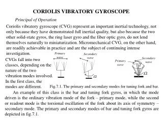
1. Secondary wave Primary wave Primary wave Secondarywave . . Fig.7.1. The primary and secondary modes for tuning fork and bar. • CORIOLIS VIBRATORY GYROSCOPE Principal of Operation Coriolis vibratory gyroscope (CVG) represent an important inertial technology, not only because they have demon­strated full inertial quality, but also because the two other solid-state gyros, the ring laser gyro and the fiber optic gyro, do not lend themselves naturally to miniaturization. Micromechanical CVG, on the other hand, are readilyachievable in practice and are the subject of continuing intense investigation. CVGs fall into two classes, depending on the nature of the two vibration modes involved. In the first class, the modes are different. An example of this class is the bar and tuning fork gyros, in which the mode driven is the ordinary vibration mode of the fork – primary mode, while the second or readout mode is the torsional oscillation of the fork about its axis of symmetry – secondary mode. The primary and secondary modes of bar and tuning fork gyros are depicted in fig.7.1.

2. In the second class, the two modes are identical, being two orthogonal modes (modes of the same natural frequency) of an axisymmetric elastic body. Examples are the vibrating prismatic (square) bar, the vibrating cylindrical and hemispherical shells, and in fact the Foucault pendulum. One mode of the pendulum, for example, can be taken as its swinging in a north-south direction, and the orthogonal mode is its swinging in an east-west direction.The operation of a coriolis vibrating gyroscope is based on sensitivity of elastic resonant structures to inertial rotation. One of the most important parameters of resonators describing its quality is Q-factor, which depends on properties of a material from which the resonator is manufactured, and also on degree of an axisymmetry of its shape etc. and is determined as: Q = o/2=f, (7.1) Where o, f is circular and cyclic natural frequency of a resonator, is timeof etimes damping of free oscillations amplitude.

3. 4 1 a b 3 2 • Fig.7.2. Conventional resonators made of fused quarts with tines (a) and modern tineless resonator (b). Internal stem; 2. External stem; 3. Hemisphere; 4. Tines Fig.7.3. Hemispherical resonator modes. n=0 n=1 n=2 n=3 • The most ideal symmetry from all geometrical figures has a sphere, therefore the most perspective sensing elements for Coriolis gyros, from a point of view of accuracy, have the hemispherical resonators made of high Q-factor material fused quarts (see fig. 7.2). The real resonator has many different natural modes of oscillations distinguished by a waveform and oscillation frequency. For the hemispherical resonator the most important natural modes are represented in a fig. 7.3.

4. q  w+(l,t) w-(l,t) o  R Fig. 7.4. Counter-propagated waves. The zero mode (n=0) corresponds to oscillations of stretching - compression, it does not take into account during CVG development as these deformations are small in comparison with flexural deformations. The first mode (n=1) corresponds to the resonator motion as rigid body. This vibration mode is excited owing to resonator stem deformation and is referred to as pendulum oscillation.It takes into account when resonator dynamic problems are under consideration. The second mode (n=2) is used as a working mode. it is the lowest flexural oscillations of the hemispherical resonator. If to excite oscillations in a thin shell by means of impact, it resonates at one of its natural modes. The waves w+(l,t) andw-(l,t) from a point of excitation q (Fig.7.4), being propagated clockwise and counterclockwise are imposed and form a standing wave: (7.2) • where n=2n/L , n=Cn, n is mode number, L is a perimeter of resonator , , , are amplitudes and phase of the counter propagated waves. For the lowest second mode n=2 of flexural oscillations, after transformations and transition from linear coordinate l to the circular one  using a ratio l=R, for real part of expression (7.2) we shall have:

5. 45о X Y Primary wave Resonator in static Secondary wave  n=2 mode Fig. 7.6. Elastic waves for n=2 mode in CVG resonator. F1 V1 Fс  F4 V2 V4 F2 V3 Fс F3 Fig. 7.5. Coriolis force inrotating resonator w2(,t)=Acos2( -o)cos2t ; (7.3) Thus, each of elementary mass moving in accordance with the simple harmonic law and is similar to Foucault pendulum i.e. tries to keep its angular momentum in inertial space at a constant value. As a result, when the shell rotates about its axis of symmetry in relation to inertial space, each elementary mass of a standing wave experiences an action of the Coriolis forces (Fig. 7.5) F1, F2, F3, F4: Fi=2[Vi](7.4) The resultant Coriolis force Fc excites an orthogonal wave (orthogonal on a circumferential angle and time phase), which nodal points coincide with antinodal points, and antinodal points with nodal points of initial wave. Elastic waves disposition in ring resonator is depicted in fig.7.6. The superposition of initial and orthogonal waves results in that the resultant wave rotates relative to its own casing and to inertial space through an angle proportional to angular rate of resonator rotation.

6. Y  X Fig.7.7. Two-dimensional pendulum. The steady-state resultant wave can be written as follows: w2(,t)=Acos2(-)cos(2t-), (7.5) where (7.6) As can be seen from expression (7.6) scale factor of the rate integrated gyro K = 0.4 (it is called Bryan coefficient). At the description of the resonator dynamics two models of oscillations are used in main: model of two-dimensional pendulum and ring model. Two-Dimensional Pendulum Model • The model of two-dimensional pendulum is shown in a fig. 7.7. The equations of motion of a two-dimensional pendulum rotating with angular rate  around the axis Z, under condition ofsmallness of 2 and , where super point means a time derivative, have the following view: (7.7)

7. Y Y Y =? 0 2 =0 o o o X X X c b a Fig. 7.8. Two-dimensional pendulum trajectory. Here  is e times damping time of free oscillations amplitude of the resonator, fx, fyis a generalized external forces acting on a pendulum. When  = 0 the pendulum trajectory in the plane XY is the direct line (see fig. 7.8а) and the oscillations represent a standing wave. When  = const  0 trajectory of the pendulum is the ellipse (fig. 7.8b), the principal axis of which makes the angle 2 with the X axis, where the angle  is determined from the last ratio of expressions (7.6). In this case standing wave has small travelling component. If a trajectory of the pendulum is the circle (fig. 7.8с), oscillations represent a pure traveling wave and the pendulum loses property to measure angular rate. Ring Model In ring model the resonator is represented by a thin elastic ring, which oscillates in a radial direction, as shown in Fig. 5.8. The equation of motion of such ring can be written as follows: (7.8) where 2= EI/(SR4); r - density of a material, E - Young's modulus, S - ring square , I - momentum of inertia of cross section relative to flexural axis, R - radius of a ring, w (, t) - radial displacement of a ring relative to its undistorted state with

8.  0о 45о 315о А' -А А -А' 270о 90о -А' А -А А' 225о 135о 180о Fig.7.10.Read-out electrodes disposition. coordinate  at a time moment t, pw, pv - external force projection on radial and tangential directions (see fig. 7.9). The super dash designates  derivative. The solution of this equation we shall find as: w(,t)=x(t)cos2+y(t)sin2 (7.9) Substitute (7.9) in (7.8), under condition that only radial force is acting ,and applying Bubnov - Galerkin method, we can obtain: (7.10) Comparing equations (7.7) and (7.10) we can see that they are identical at k=0.4. Thus ring model and two-dimensional pendulum model describe physical processes in CVG with equal accuracy. Read-out System The measurement system of turning angle  of wave pattern consists of eight electrodes symmetrically located along a circle, each of which is connected to a diametrically opposite electrode (see fig.5.10). Such arrangement of pickoff electrodes is necessary in a case, when the second mode is used as a working one. The second mode has a property to divide a shell onto a parts spaced through angle 180о, which are equally moved.

9. Each electrode is electrically connected to an electrode spaced from it through the angle 180о. The electrode in 0о position is connected to an electrode in 180о position (designated on a figure by the A' ) the electrode in 90о position is connected to an electrode 270о (designated as -A') etc. The mode n = 2 has also the following property: when mass points of the resonator located at 0о and 180о is moving from electrode, mass point located at 90о and 270о is moving to an electrode. These four electrodes of a read-out system will form only one information channel. The cosine channel of a signal Еc is obtained by joining of amplified signals A' and -А ' in a difference amplifier. The second informative channel, sine channel, Еs, is similarly obtained by subtraction of signals from electrodes located on 45o, 225o and 135o, 315o. The required turn angle of a wave pattern is determined as half of arctangent of the relation of amplitudes of sine and cosine channels: (7.11 ) are demodulated signals of sine and cosine channels, respectively. Parametric Excitation (rate integrated gyro) Let's consider a problem of excitation and control of a standing wave. First of all it should be noted, that the energy losses of oscillations in a quartz resonator are extremely small. The stationary value of resonator damping time  is a time necessary to damp oscillation frequency of the resonator е times from its initial value is large enough.

10. Voltage on Voltage off Voltage on Voltage off Ring electrode resonator Fig.7.11. Ring electrode principal of operation For example, damping time of standing wave in quartz resonators of different diametersare: 58 mm - 1800 sec, 30 mm - 1000 sec, 15 mm - 110 sec. The damping, though small, should be cancelled for stabilization of fixed value of amplitude. It is not recommended to be done by voltage applied on a pair of discrete electrodes, because it results in pulling a standing wave to these electrodes. It is necessary, that the standing wave could move freely and responded only to rotation of the gyro relative to inertial space. The method selected for compensation of damping losses consists in applying on a ring excitation electrode, alternating voltage with frequency 2 times more, than the resonance Fig. 7.11 shows the ring excitation electrode, which is located on a hemispherical casing of a gyro along circumferencial coordinate approximately from latitude 25о to 45о . When the separate parts of the device is assembled, a ring electrode and resonator form a part of a concentric-sphere capacitor. With nominal distance between plates of 0.15 mm. When the ring capacitor: the electrode - resonator is charged from a source and the resonator is not deformed, the electrical forces are radially symmetric and are identical by value. In this case there is not a resultant force acting on the mode n = 2.

11. However, when the resonator is deformed, per square force with a smaller gap increases, and in a region with a larger gap decreases. As a result a resultant force arises making the resonator to be deformed even more and this force is directed along the line passing through antinodes. Four wave configurations shown in fig.7.11 illustrate a principle of excitation. In the first, the resonator is deforming in the direction of its maximum deformation. The voltage is on and work is being done on the mode n = 2. In the second portion, the resonator is returning to the spherical shape and the voltage is off. In the third and fourth portions the voltage is sequentially repeated.