Chi-Square Applications
Chi-Square Applications. Chapter 15. GOALS. List the characteristics of the chi-square distribution . Conduct a test of hypothesis comparing an observed set of frequencies to an expected distribution. Conduct a test of hypothesis to determine whether two classification criteria are related.


Chi-Square Applications
E N D
Presentation Transcript
Chi-Square Applications Chapter 15
GOALS • List the characteristics of the chi-square distribution. • Conduct a test of hypothesis comparing an observed set of frequencies to an expected distribution. • Conduct a test of hypothesis to determine whether two classification criteria are related.
Characteristics of the Chi-Square Distribution The major characteristics of the chi-square distribution are: • It is positively skewed. • It is non-negative. • It is based on degrees of freedom. • When the degrees of freedom change a new distribution is created.
Goodness-of-Fit Test: Equal Expected Frequencies • Let f0 and fe be the observed and expected frequencies respectively. • H0: There is no difference between the observed and expected frequencies. • H1: There is a difference between the observed and the expected frequencies.
Goodness-of-fit Test: Equal Expected Frequencies The test statistic is: The critical value is a chi-square value with (k-1) degrees of freedom, where k is the number of categories
Goodness-of-Fit Example Ms. Jan Kilpatrick is the marketing manager for a manufacturer of sports cards. She plans to begin selling a series of cards with pictures and playing statistics of former Major League Baseball players. One of the problems is the selection of the former players. At a baseball card show at Southwyck Mall last weekend, she set up a booth and offered cards of the following six Hall of Fame baseball players: Tom Seaver, Nolan Ryan, Ty Cobb, George Brett, Hank Aaron, and Johnny Bench. At the end of the day she sold a total of 120 cards. The number of cards sold for each old-time player is shown in the table on the right. Can she conclude the sales are not the same for each player? Use 0.05 significance level.
Step 1: State the null hypothesis and the alternate hypothesis. H0: there is no difference between fo and fe H1: there is a difference between fo and fe Step 2: Select the level of significance. α = 0.05 as stated in the problem Step 3: Select the test statistic. The test statistic follows the chi-square distribution, designated as χ2
Step 5: Compute the value of the Chi-square statistic and make a decision
34.40 The computed χ2 of 34.40 is in the rejection region, beyond the critical value of 11.070. The decision, therefore, is to reject H0 at the .05 level . Conclusion: The difference between the observed and the expected frequencies is not due to chance. Rather, the differences between f0 and fe and are large enough to be considered significant. It is unlikely that card sales are the same among the six players.
Goodness-of-Fit Test: Unequal Expected Frequencies • Let f0 and fe be the observed and expected frequencies respectively. • H0: There is no difference between the observed and expected frequencies. • H1: There is a difference between the observed and the expected frequencies.
Goodness-of-Fit Test: Unequal Expected Frequencies - Example The American Hospital Administrators Association (AHAA) reports the following information concerning the number of times senior citizens are admitted to a hospital during a one-year period. Forty percent are not admitted; 30 percent are admitted once; 20 percent are admitted twice, and the remaining 10 percent are admitted three or more times. A survey of 150 residents of Bartow Estates, a community devoted to active seniors located in central Florida, revealed 55 residents were not admitted during the last year, 50 were admitted to a hospital once, 32 were admitted twice, and the rest of those in the survey were admitted three or more times. Can we conclude the survey at Bartow Estates is consistent with the information suggested by the AHAA? Use the .05 significance level.
Goodness-of-Fit Test: Unequal Expected Frequencies - Example Step 1: State the null hypothesis and the alternate hypothesis. H0: There is no difference between local and national experience for hospital admissions. H1: There is a difference between local and national experience for hospital admissions. Step 2: Select the level of significance. α = 0.05 as stated in the problem Step 3: Select the test statistic. The test statistic follows the chi-square distribution, designated as χ2
Expected frequencies of sample if the distribution stated in the Null Hypothesis is correct Distribution stated in the problem Frequencies observed in a sample of 150 Bartow residents Computation of fe 0.40 X 150 = 60 0.30 X 150 = 45 0.30 X 150 = 30 0.10 X 150= 15
Computed χ2 Step 5: Compute the value of the Chi-square statistic and make a decision
1.3723 The computed χ2 of 1.3723 is in the “Do not reject H0” region. The difference between the observed and the expected frequencies is due to chance. We conclude that there is no evidence of a difference between the local and national experience for hospital admissions.
Contingency Table Analysis Acontingency tableis used to investigate whether two traits or characteristics are related. Each observation is classified according to two criteria. We use the usual hypothesis testing procedure. • The degrees of freedomis equal to: (number of rows-1)(number of columns-1). • The expected frequency is computed as:
Contingency Analysis We can use the chi-square statistic to formally test for a relationship between two nominal-scaled variables. To put it another way, Is one variable independent of the other? • Ford Motor Company operates an assembly plant in Dearborn, Michigan. The plant operates three shifts per day, 5 days a week. The quality control manager wishes to compare the quality level on the three shifts. Vehicles are classified by quality level (acceptable, unacceptable) and shift (day, afternoon, night). Is there a difference in the quality level on the three shifts? That is, is the quality of the product related to the shift when it was manufactured? Or is the quality of the product independent of the shift on which it was manufactured? • A sample of 100 drivers who were stopped for speeding violations was classified by gender and whether or not they were wearing a seat belt. For this sample, is wearing a seatbelt related to gender? • Does a male released from federal prison make a different adjustment to civilian life if he returns to his hometown or if he goes elsewhere to live? The two variables are adjustment to civilian life and place of residence. Note that both variables are measured on the nominal scale.
Contingency Analysis - Example The Federal Correction Agency is investigating the last question cited above: Does a male released from federal prison make a different adjustment to civilian life if he returns to his hometown or if he goes elsewhere to live? To put it another way, is there a relationship between adjustment to civilian life and place of residence after release from prison? Use the .01 significance level.
Contingency Analysis - Example The agency’s psychologists interviewed 200 randomly selected former prisoners. Using a series of questions, the psychologists classified the adjustment of each individual to civilian life as outstanding, good, fair, or unsatisfactory. The classifications for the 200 former prisoners were tallied as follows. Joseph Camden, for example, returned to his hometown and has shown outstanding adjustment to civilian life. His case is one of the 27 tallies in the upper left box (circled).
Contingency Analysis - Example Step 1: State the null hypothesis and the alternate hypothesis. H0:There is no relationship between adjustment to civilian life and where the individual lives after being released from prison. H1:There is a relationship between adjustment to civilian life and where the individual lives after being released from prison. Step 2: Select the level of significance. α = 0.01 as stated in the problem Step 3: Select the test statistic. The test statistic follows the chi-square distribution, designated as χ2
Contingency Analysis - Example Step 4: Formulate the decision rule.
(120)(50) 200 Computing Expected Frequencies (fe)
5.729 Conclusion The computed χ2 of 5.729 is in the “Do not reject H0” region. The null hypothesis is not rejected at the .01 significance level. Conclusion: There is no evidence of a relationship between adjustment to civilian life and where the prisoner resides after being released from prison. For the Federal Correction Agency’s advisement program, adjustment to civilian life is not related to where the ex-prisoner lives.