Download
1 / 48
510 likes | 915 Views
Hydraulic Transients. When the Steady-State design fails!. gradually. varied. Hydraulic Transients: Overview. In all of our flow analysis we have assumed either _____ _____ operation or ________ ______ flow What about rapidly varied flow? How does flow from a faucet start?

E N D
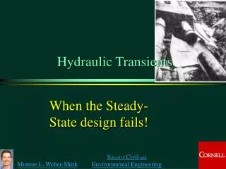
Hydraulic Transients When the Steady-State design fails!
gradually varied Hydraulic Transients: Overview • In all of our flow analysis we have assumed either _____ _____ operation or ________ ______ flow • What about rapidly varied flow? • How does flow from a faucet start? • How about flow startup in a large, long pipeline? • What happens if we suddenly stop the flow of water through a tunnel leading to a turbine? steady state
Hydraulic Transients Unsteady Pipe Flow: time varying flow and pressure • Routine transients • change in valve settings • starting or stopping of pumps • changes in power demand for turbines • changes in reservoir elevation • turbine governor ‘hunting’ • action of reciprocating pumps • lawn sprinkler • Catastrophic transients • unstable pump or turbine operation • pipe breaks
References • Chaudhry, M. H. 1987. Applied Hydraulic Transients. New York, Van Nostrand Reinhold Company. • Wylie, E. B. and V. L. Streeter. 1983. Fluid Transients. Ann Arbor, FEB Press.
Analysis of Transients • Gradually varied (“Lumped”) _________ • conduit walls are assumed rigid • fluid assumed incompressible • flow is function of _____ only • Rapidly varied (“Distributed”) _________ • fluid assumed slightly compressible • conduit walls may also be assumed to be elastic • flow is a function of time and ________ ODE time PDE location
Establishment of Flow:Final Velocity How long will it take? 1 g = 9.8 m/s2 H = 100 m K = ____ f = 0.02 L = 1000 m D = 1 m 1.5 H EGL HGL V 2 0.5 L Ken= ____ Kexit= ____ 1.0 minor major
Final Velocity g = 9.8 m/s2 H = 100 m K = 1.5 f = 0.02 L = 1000 m D = 1 m 9.55 m/s What would V be without losses? _____ 44 m/s
Establishment of Flow:Initial Velocity before head loss becomes significant 10 9 g = 9.8 m/s2 H = 100 m K = 1.5 f = 0.02 L = 1000 m D = 1 m 8 7 6 velocity (m/s) 5 4 3 2 1 0 0 5 10 15 20 25 30 time (s)
Flow Establishment:tanh! V < Vf
Time to reach final velocity Time to reach 0.9Vf increases as: L increases H decreases Head loss decreases
Flow Establishment g = 9.8 m/s2 H = 100 m K = 1.5 f = 0.02 L = 1000 m D = 1 m Was f constant?
Household plumbing example • Have you observed the gradual increase in flow when you turn on the faucet at a sink? • 50 psi - 350 kPa - 35 m of head • K = 10 (estimate based on significant losses in faucet) • f = 0.02 • L = 5 m (distance to larger supply pipe where velocity change is less significant) • D = 0.5” - 0.013 m • time to reach 90% of final velocity? T0.9Vf = 0.13 s
Lake Source Cooling Intake Schematic Motor Lake Water Surface Steel Pipe 100 m ? Plastic Pipe 3100 m Intake Pipe, with flow Q and cross sectional area Apipe 1 m Pump inlet length of intake pipeline is 3200 m Wet Pit, with plan view area Atank What happens during startup? What happens if pump is turned off?
Q Transient with varying driving force where Lake elevation - wet pit water level H = ______________________________ f(Q) What is z=f(Q)? Finite Difference Solution! Is f constant?
Wet Pit Water Level and Flow Oscillations constants What is happening on the white vertical lines?
Wet Pit with Area Equal to Pipe Area Pipe collapse Water Column Separation Why is this unrealistic?
Period of Oscillation: Frictionless Case z = -H z = 0 at lake surface Wet pit mass balance
Period of Oscillations plan view area of wet pit (m2) 24 pipeline length (m) 3170 inner diameter of pipe (m) 1.47 gravity (m/s2) 9.81 T = 424 s
Transients • In previous example we assumed that the velocity was the same everywhere in the pipe • We did not consider compressibility of water or elasticity of the pipe • In the next example water compressibility and pipe elasticity will be central
infinite force Valve Closure in Pipeline V • Sudden valve closure at t = 0 causes change in discharge at the valve • What will make the fluid slow down? • Instantaneous change will require _______ _______ • Impossible to stop all the fluid instantaneously What do you think happens?
Transients: Distributed System • Tools • Conservation of mass • Conservation of momentum • Conservation of energy • We’d like to know • pressure change • rigid walls • elastic walls • propagation speed of pressure wave • time history of transient
Pressure change due to velocity change HGL steady flow unsteady flow velocity density pressure
Momentum Equation HGL 1 2 Mass conservation A1 A2 Dp = p2 - p1
Magnitude of Pressure Wave 1 2 Increase in V causes a _______ in HGL. decrease
Propagation Speed:Rigid Walls Conservation of mass Solve for DV
Propagation Speed:Rigid Walls momentum mass Need a relationship between pressure and density!
Propagation Speed:Rigid Walls definition of bulk modulus of elasticity Example: Find the speed of a pressure wave in a water pipeline assuming rigid walls. (for water) speed of sound in water
Propagation Speed:Elastic Walls D Additional parameters D = diameter of pipe t = thickness of thin walled pipe E = bulk modulus of elasticity for pipe effect of water compressibility effect of pipe elasticity
Propagation Speed:Elastic Walls • Example: How long does it take for a pressure wave to travel 500 m after a rapid valve closure in a 1 m diameter, 1 cm wall thickness, steel pipeline? The initial flow velocity was 5 m/s. • E for steel is 200 GPa • What is the increase in pressure? solution
Time History of Hydraulic Transients: Function of ... • Time history of valve operation (or other control device) • Pipeline characteristics • diameter, thickness, and modulus of elasticity • length of pipeline • frictional characteristics • tend to decrease magnitude of pressure wave • Presence and location of other control devices • pressure relief valves • surge tanks • reservoirs
Time History of Hydraulic Transients 1 3 DH DH V=Vo V=0 V= -Vo V=0 a a L L 2 4 DH V=0 V= -Vo L L
Time History of Hydraulic Transients 5 7 DH DH V= -Vo V=Vo V=0 V=0 a a L L 6 8 DH V= Vo V=0 L L
Pressure variation over time DH Pressure head reservoir level Neglecting head loss! time Pressure variation at valve: velocity head and friction losses neglected
Lumped vs. Distributed For _______ system lumped • For LSC wet pit • T = 424 s • L/a = 3170 m/1400 m/s = ____ pressure wave period T = _________________ 2.3 s
Methods of Controlling Transients • Valve operation • limit operation to slow changes • if rapid shutoff is necessary consider diverting the flow and then shutting it off slowly • Surge tank • acts like a reservoir closer to the flow control point • Pressure relief valve • automatically opens and diverts some of the flow when a set pressure is exceeded
Surge Tanks • Reduces amplitude of pressure fluctuations in ________ by reflecting incoming pressure waves • Decreases cycle time of pressure wave in the penstock • Start-up/shut-down time for turbine can be reduced (better response to load changes) Reservoir Surge tank Tunnel/Pipeline Penstock tunnel T Tail water Surge tanks
Use of Hydraulic Transients • There is an old technology that used hydraulic transients to lift water from a stream to a higher elevation. The device was called a “Ram Pump”and it made a rhythmic clacking noise. • How did it work? High pressure pipe Source pipe Stream Ram Pump
Burst section of Penstock:Oigawa Power Station, Japan Chaudhry page 17
Collapsed section of Penstock:Oigawa Power Station, Japan Chaudhry page 18
Values for Wet Pit Analysis Flow rate before pump failure (m3/s) 2 plan view area of wet pit (m2) 24 pipeline length (m) 3170 inner diameter of pipe (m) 1.47 elevation of outflow weir (m) 10 time interval to plot (s) 1000 pipe roughness (m) 0.001 density (kg/m3) 1000 dynamic viscosity (Ns/m2) 1.00E-03 gravity (m/s2) 9.81
Pressure wave velocity: Elastic Pipeline E = 200 GPa D = 1 m t = 1 cm 0.5 s to travel 500 m
Ram Pump Air Chamber Rapid valve Water inlet
Ram pump H2 High pressure pipe Source pipe Stream H1 Ram Pump
Ram Pump Time to establish flow