Transients in 3ph CCTs
Transients in 3ph CCTs. Two methods: 1-extension of 1ph approach 2-Sym Components The 1 st emphasized, physical picture Type of Neutral Connection: 1-solidly Gr 2-Isolated 3-Neutral Impedance .

Transients in 3ph CCTs
E N D
Presentation Transcript
Transients in 3ph CCTs • Two methods: 1-extension of 1ph approach 2-Sym Components The 1st emphasized, physical picture • Type of Neutral Connection: 1-solidly Gr 2-Isolated 3-Neutral Impedance
Isolated Neutral Vs Solidly Gr • TRV in 3ph, Is. N. Sys, ~ TRV 1ph • In this 3ph CCT : TRV-peak=2√(2/3) V each ph. as clear • In 3ph CCT,Iso. N.: Balanced:O close to N □In Sw. 1st A open & Load N shift to P □VAP across phase A C.B.:√3V/2 & during transient, peak= 2√2x√3 V/2=√ 6 V □50% more than: 3ph with neutral Gr
3ph Isolated N, load disconnecton • 2 other Phs interrupt shortly after A • duties less sever, since 2ph in series with 2 breaks to open under V • In unGr N, duty of 1st ph to clear 3ph fault is the most severe • In Gr N, 3 poles of C.B. identical duty
Switching 3ph Reactor, Iso. N. • open 3 ph reactor load L /ph, & stray C/ph, with Π model • N Gr through 3C □ If A open 1st: VA neg. Max, VB & VC Pos. half peak; C rising, B falling • Variation of I & V, 3ph • VBC=0 this instant, IB=-IC, peak :√3/2 I
Reactor, Iso. N. switching • IB & IC when, IA interrupt, have sudden slope change & zero in a 90◦ • VBC derive I & now is zero, and 90◦ later at peak □ CCT is Sym. & if fold □Then Solve it for VAA’ by injecting opp. I to it, FIG
Rearrangement of CCT • After folding CCT • CCT of this FIG examined in (3.4) • TRV of 2nd & 3rd pole, same method • Equal I inj. at BB’ & CC’ for simulation • And Simplified CCT
CCT, 2nd & 3rd poles interrupt • Simulation CCT & Effective one • f =1/[2Π√LC] • An example of 3ph motor interruption
3ph Capacitance Switching • Cap. with unground N & isolated from source • S.S. , N at G level • CN discharged • A interrupt 1st IA0, VA peak IBC=IB=-IC=√3/2.Vp ωC • VB=VC=-Vp/2 • IBC max0, 1/4cycle • Case 1: B&C open VBC√3 VP (its peak)
Discussion Continued • this I charge CB and discharge Cc rise of VN & current flow to CN • Charge added to CB & removed from Cc Q=∫I dt=√3/2.VpωC∫cosωt =√3/2 Vp C t=0Π/2ω □ Change in potential of CB&CC: √3 Vp/2 □ Voltage on the Bank as in FIG
Voltage Trapped & Phasor Diag. • CCT, after breaker open in B&C,1/4cycle □ After ¼ cycle VB=√3/2 Vp • CN<<C its current negligible • VN=VB-Vp(-1/2+√3/2)=Vp/2
Max Voltages across CB contacts • High Voltages across C.B.restrikes • by Trapped charges, one side fixed , • The other driven by supply, their max: VA=2.5Vp (90◦ after B&C clear), VB=(1+√3/2)Vp (210◦ after B&C clear) VC=(1+√3/2)Vp(150◦ after B&C clear) □ Case 2: B&C do not interrupt in 90◦ after A □Voltage VAA’=VAC-VA’C’ assuming C not interrupted: □C &C’ at same potential, VA’N=Vp
Case 2, Discussion continued • VA’C’=VA’N+VNC’, • initially VNC’=0.5Vp • Then half of ph-ph voltage: VBC=√3 Vp sinωt VNC’=Vp(0.5+√3/2 sinωt) and : VA’C’=Vp(1.5+√3/2sinωt) • At source: VAC=√3Vpsin(ωt+Π/3)= =√3Vp(1/2sinωt+√3/2cosωt) VAA’=VAC-VA’C’=1.5Vp(cosωt-1)
Case 2, Continued … • !80◦ later, 3Vp on A,if B&C not open • Against 2.5Vp when B&C opened • If C.B. can not withstand the Voltage across it: a- 1 or 2 contacts restrike & pass I • In 3ph Cap. Bank (isol. N) A cleared 1st , B&C after 90◦ (as case 1) then ph A restrike when VAA’=2.5Vp
Restrike on Ph.A after B&C clear • Equivalent CCT: • Initial conditions: Vs=-Vp,VCA=VA’N=+Vp VCN=VNG=0.5Vp • Voltage on CA Osc. f=1/[2Π√LCeq] Ceq=CACN/[CA+CN] • CA>>CN, • f0≈1/2Π√LCN
The Transient Current • I=2.5Vp/[√L/Ceq] sinω0t • since N swing to -4.5Vp at P on fig • corresponds to zero value in H.F. current • If C.B. clear a H.V. remain on CN & often B and C restrike • Swing of N, B’ & C’ swing by CB & Cc • When VNG 4.5 Vp VB’G=[-4.5+(√3/2-1/2)]Vp=-4.134Vp VC’G=[-4.5+(-1/2-√3/2)]Vp=-5.866Vp
Discussion continued…. • Now : VBG=0.5Vp=VCG therefore: VB’B=-4.634Vp, VCC’=-6.366Vp • one of phases likely to restrike, VLL across 2ph of bank • As if A & C closed simultaneously • Cap.Series CA & CC = ½ CA,induc=2L • ∆V=2x(sum voltages on breaks A &C) = 2x(2.5+1.366)Vp If initial restrike on pole A occur, when Vp across it
Discussion on Restrike Continued… • This Shared equally CA & CC • CN<<CA not always prevail, i.e.: O.C. Transmission Line • Considerable Cap. To Gr. & as well as phases • Where C1/C0>1 Reach one asympt. As C0 rise Effect shown on TRV of Fig □C1/C0=1 when solidly Gr
Discussion on CN Value & Effect • In Solidly Gr.:Vmax<2 PU (or in 1 ph) • Vmax=3 PU, Isolated N (function of C1/C0) • Affect the restrike of C.B. • 1 Ph. SW. analysis Principals employed □ Symmetrical Components Method
The Symmetrical Component • Asymmetry removed by : replacing it, 3 sequence Network synthesize asymmetrical comp.s • Fortescue: extension, Transient study • Osc. freq. resolved in +,-,0 seq. comp • Voltages Asymm. When ph A of C.B. opens • VA,VB,VC have Sym comp. V0,V1,V2 • Opening A • ~ inserting Z between Contacts • Z∞ ≡ interrupting current
CCT Breaker Interruption & Fault • A 3 Ph Fault &1stpole Opens • (if a=e^j2Π/3) & • VA=IAZ, VB=Vc=0 • V0=1/3(VA+VB+Vc) V1=1/3(VA+aVB+VC) V2=1/3(VA+aVB+aVC) • V0=V1=V2=VA/3 • I0+I1+I2=VA/Z
Sym. Comp. for Transient Analysis • V0=I0Z0,V1=I1Z1+E1, V2=I2Z2 • Seq. Imp. seen from one ph. Contacts • or 3V0=3V1=3V2=VA • 3V0=I03Z0, 3V1=I13Z1+3E1,3V2=I23Z2 • VA across C.B. is TRV • When 2nd &3rd open similar CCT can be proposed • Not well adapted to: Assym. Faults
Sym. Comp. Application …. • Viewed from contacts, not a balanced system • 2 Degrees of Asym.(Fault&Switch) • In Case of 1 ph to Gr Fault: Seq. Network as Fig. • As seen from Fault rather than breaker • Iloop=IF/3=I0=I1=I2 • Just if C.B. in branch develop across it & TRV across it
Discussion of Seq. Comp. ph-G F • Network so Connected : seq. voltages add • C.B. clearing F not at F& elsewhere • Switches should opened simult. In 3 Networks • Seq. comp. currents must be injected at C.B. terminals in each ph seq. • TRV of C.B. is the sum of these 3 responses
Practical Application • 1 ph-Gr F on a Cable System • The Eq. CCT • The seq. Network of fault needed • CQ:Iso-NCapBank CR: Neutral Cap. • CP: Cable cap./phase • L:source inductance
Seq. Network of 1 Ph._Gr F • The Seq. Network • To apply Current Injection, E sh.cct. • Then remaining CCT Reduced simple CCT(2 Freq) • CR<<CQ & CP Then C0=Cp ω1=1/√[L(CP+CQ)], ω2=1/√LC0
The current Injection • Ramp Current I’t inj. Parallel LC CCT V=I’L(1-cosωt) • I’, slope of current at zero,sym F Vp/L • V=Vp(1-cosω0t) • Now Inj I0=I1=I2=1/3 IFault,SOLUTION: • V=2Vp/3(1-cosω1t)+Vp/3(1-cosω2t) • If N Gr with,4<R<20Ωs,2000>IF>400 • this affect Zero seq. network • Typical values:L=1mH,C≈5 μF • Z0=√L/C0=√1000/5=14.1Ω, • If R>28Ω Osc TRV suppressed, Fault Current control at Neutral
Sym. Comp. Solution, Discussion • load rep. by resistance contr. Damp • Load N isol. Shunt + & - seq. networks only • Compare with classical method • The injected CCT • result of it=the seq network injection
Traveling Waves & Transmission Line Model • example of Distributed parameter of: R, L, C • Phenomena of energizing a line • Travels with finite speed of EM Ws • If after ∆t a length ∆x is charged • C , F/m Q=C V ∆X
Electromagneitc Propagation • Results in : 1- An Electric Field in ∆X 2- A Magnetic Field around Cable • The current determined: I=VC∆X/∆t=CV dx/dt (dx/dt=ν) • I=CV.v • flux linkage : Φ=L∆X I =L∆X.CV.v • induced emf : (v=1/√LC) dΦ/dt=LCV v ∆X/∆t=LCV v V=LCV v2
Transmission Line Fields • Z0=√(L/C) (typical line 400Ω, Cable 30-80Ω) • A Voltage Traveling wave & then V/Z0 A Current wave • VI 1/2CV2. v and 1/2LI2 .v (each ½ VI) • P=E X H magnitude & Direction of Energy Flow
WAVE EQUATION • Small Segment • -∆V=L ∆X ∂I/∂t • ∂V/∂X=-L ∂I/∂t • current to ∆C is : -∆I=CV∆X ∂V/∂t • ∂I/∂x=-C ∂V/∂t • Combining them: ∂V/∂x=-L∂I/(∂X∂t) ∂I/∂x ∂t=-C∂V/∂t • ∂V/∂X=LC∂V/∂t • ∂I/∂x=LC∂I/∂t
SOLUTION of WAVE EQUATION • I=f[x ±1/√LC] • I(x,t)=f1(x-vt)+f2(x+vt) • employing: ∂V/∂x=-L∂I/∂t= Lv[f’1(x-vt)+f’2(x+vt)] • V(x,t)=Lv[f1(x-vt)-f2(x+vt)]= Z0 f1(x-vt)-Z0 f2(x+vt) • Combing : • V(x,t)+Z0 I(x,t)=2Z0 f1(x-vt) • V(x,t)-Z0 I(x,t)=-2Z0 f2(x+vt)