Spatial Referencing Basics: Understanding Topology & Relationships
Learn principles of spatial referencing, topological consistency, types of spatial relationships, map projections, and basic coordinate systems for Geographic Information Systems.

Spatial Referencing Basics: Understanding Topology & Relationships
E N D
Presentation Transcript
GIS in the Sciences ERTH 4750 (38031) Spatial Referencing Xiaogang (Marshall) Ma School of Science Rensselaer Polytechnic Institute Tuesday, February 05, 2013
Review of last week’s work • In the lecture • Geographic phenomena: fields and objects • Computer representations: raster and vector • Autocorrelation and topology • In the lab: MapInfo Professional • Map objects: text, points, lines and polygons • Objects layers, tables maps • Analyzing data: queries & thematic Maps • Questions?
Topology and spatial relationships The striped area is the interior of feature A • We want to find all possible relationships between two polygons for two-dimensional space • We can use the topological properties of interior and boundary to define relationships between spatial features Boundary of feature A
Eight spatial relationships A disjoint B A contains B A A B B A B A A meets B A equal B B A B B A overlap B A covered by B A A A B B A covers B A inside B
Five rules of topological consistency Rule 1 • Every line must be bounded by two nodes • Every line borders two polygons, namely the left and the right polygon • Every polygon has a closed boundary consisting of an alternating (and cyclic) sequence of points and lines • Around every point exists an alternating (and cyclic) sequence of lines and polygons • Lines only intersect at their bounding nodes Rules 2, 5 Rule 3 Rule 4 Understand the ‘line’ here as a part of the boundary of a polygon
Understand the ‘line’ here as a part of the boundary of a polygon Then, the rule 5 ‘Lines only intersect at their bounding nodes’ also indicates that the current lines are dividable, see the example at left, we can divide a line into three by adding another polygon.
Acknowledgements • This lecture is partly based on: • Huisman, O., de By, R.A. (eds.), 2009. Principles of Geographic Information Systems. ITC Press, Enschede, The Netherlands
Outline • Spatial referencing basics • Map projections
1 Introduction • Spatial referencing encompasses the definitions, the physical/geometric constructs and the tools required to describe the geometry and motion of objects near and on the Earth’s surface • Some of these constructs and tools are usually itemized in the legend of a published map
1 Introduction Legend of a German topographic map 11
2 Spatial referencing basics • International Terrestrial Reference System – the origin is in the center of the mass of the Earth. This system rotates together with the Earth. Used in extra-terrestrial positioning systems, like GPS • International Terrestrial Reference Frame – a set of points with high precision location and speed definition (a triangle-based network). The speed expresses the change of location in time due to geophysical (e.g. tectonic) phenomena
2.1 Basic coordinate systems Geographic coordinates – Two-dimensional coordinate system, referring to locations on (or close to) the surface of the Earth, using angles for defining locations Cartesian coordinates – Rectangular coordinate system, using linear distance for defining locations on a plane
2.2 Shape of the Earth • Development of the ideas about the shape of the Earth: • An oyster (The Babylonians before 3000 BC) • A circular disk (early antiquity; approximately 5-300 B.C., but this concept survived till the 19thcentury) • A very round pear (Christopher Columbus in the last years of his life) • A perfect ball a sphere (Pythagoras in 6thcentury BC) • An ellipsoid, flattened at the poles (Newton around the turn of the 17th and 18th centuries) • …but what is it exactly? Modeling the shape of the Earth is needed for spatial referencing. In this sense, topographic differences (e.g., mountains and lowlands) are not taken into account. 14
2.2 Shape of the Earth • The geoid • The surface of the Earth is irregular and continuously changing in shape due to irregularities in mass distribution inside the earth. • Geoid: An equipotential surface in the gravity field of our planet; a ‘potato’ like shape, which is ever changing, although relatively slowly. • Every point on the geoid has the same zero height all over the world.
2.3 Datums • For spatial referencing we need a datum: a surface that represents the shape of the earth. • Due to practical reasons, two types of spatial positioning are considered: • Computing elevations (related to a vertical datum), • Computing horizontal positions (related to a horizontal datum). Source of clip art: http://www.school-clip-art.com
2.3.1 Vertical datum • A reference surface for heights (vertical datum) must be: • a surface of zero height, • measurable (to be sensed with instruments), • level (i.e. horizontal). • The geoid is practically the most obvious choice: • the geoid is approximately expressed by the surface of all the oceans of the Earth (mean sea level), • every point on the geoid has the same zero height all over the world.
Mean sea level = geoid? • Mean Sea Level (MSL) is used as zero altitude • the ocean’s water level is registered at coastal locations over several years • Sea level at the measurement location is affected by tidal differences, ocean currents, winds, water temperature and salinity • Many local vertical datums exist • Different countries, different vertical datums. • E.g.: MSLBelgium-2.34 m = MSLNetherlands Tide table of Isle aux Morts (Canada). Sea surface changes predictably but irregularly. Source: http://www.lau.chs-shc.dfo-mpo.gc.ca/cgi-bin/tide-shc.cgi 18
Vertical datum in the United States • The North American Vertical Datum of 1988 (NAVD88) Its inscription reads "State of Colorado / 2003 Mile High Marker / 5280 Feet Above Sea Level / NAVD 88". Elevation marker at The Colorado State Capitol Source: http://www.mesalek.com/colo/trivia/elev.html
Highest and lowest points in the US • Lowest point: Death Valley, Inyo County, California −282 ft (−86 m) below sea level • Highest point: Mount McKinley, Denali Borough, Alaska +20,320 ft (6,194 m) above sea level Source: http://en.wikipedia.org/wiki/Geography_of_the_United_States 20
Elevation measurement from the vertical datum • Starting from MSL points, the heights of points on the Earth can be measured using geodetic leveling techniques
Geoid versus ellipsoid • The geoid surface continuously changes in shape due to changes in mass density inside the earth (i.e. it is a dynamic surface). • Due to its dynamics and irregularities, geoid is NOT SUITABLE for defining time-indifferent elevations (as well as it is not a suitable reference surface for the determination of locations, see later). • A (regular) mathematical vertical datum is needed. • The best approximation of the geoid is an ellipsoid. Note that if a=b then it is a sphere. Rotation of this ellipse around the minor axis gives the ellipsoid
Comparison of vertical datums • Elevations measured from different datums are different, thus, the datum has to be known for proper georeferencing.
2.3.2 Horizontal datum • For local measurements, where the size of the area of interest does not exceed 10 km, a plain is a proper horizontal datum for most of the applications. • For applications related to larger areas the curvature of the Earth has to be considered. • Mathematically describable surface: ellipsoid (sphere). Note that the ellipsoid is not a plain. A map projection has to be applied (see later in this lecture) to represent the points on the ellipsoid in the plain of the map.
Local horizontal datums • Countries establish a horizontal datum • an ellipsoid with a fixed position, so that the ellipsoid best fits the surface of the area of interest (the country) • topographic maps are produced relative to this horizontal (geodetic) datum • Horizontal datum is defined by the size, shape and position of the selected ellipsoid: • dimensions (a, b) of the ellipsoid • the reference coordinates (φ, λ and h) of the fundamental point • angle from this fundamental point to another point 25
Hundreds of local horizontal datums do exist Most widely used datum-ellipsoid pairs Courtesy: https://www.navigator.navy.mil
Local and global datums Local and global ellipsoids related to the geoid. The shapes are exaggerated for visual clarity. 27
Local and global datums • Attempts to come to one single global horizontal AND vertical datum: • Geodetic Reference System 1980 ellipsoid (GRS80) • accurate global geoid in near future? • Among difficulties: • accurate determination of one ‘global’ height • from hundreds of local datums to one global datum • If successful: • GIS users don’t have to bother about spatial referencing and datum transformation any more
Commonly used ellipsoids These selected ellipsoids are listed here as an example. There is no contradiction between this list and the figure in slide 18, since in all the regions several ellipsoids are used.
Horizontal datums - example Datum: ellipsoid with its location. Note that the above ellipsoids are the same, but their positions are different.
2.3.3 Datum transformations • Why ? • For the transformation of map coordinates from one map datum to another • What ? • Transformation between two Cartesian spatial reference frames • How ? • Transformation parameters (shift and modify ellipsoid) • Rotation angles (α, β, γ) • Translation (origin shift) factors (X0, Y0, Z0) • Scaling factor (s) 31
3 Map projections • The curved surface of the Earth (as modeled by an ellipsoid) is mapped on to a flat plane using a map projection. • Two reference surfaces are applied: • Ellipsoid for large-scale mapping (e.g. 1:50,000) • Sphere for small-scale mapping (e.g. 1:5,000,000) See also: http://www.bbc.co.uk/history/british/empire_seapower/launch_ani_mapmaking.shtml
3.1 Classes of map projections • Surfaces used for projecting the points from the horizontal reference surface (datum) onto are: • plane or • a surface that can be deduced to a plane: • cone • cylinder • Any other (closed) body that consists of planes can be also used (e.g. a cube), but those are mostly of limited practical value.
Secant projections • In tangent projections the projection surfaces touch the reference surface in one point or along a closed line. • In secant projections the projection surface intersect the reference surface in one or two closed lines.
A transverse and an oblique projection • Normal projection: α=0º • Transverse projection: α=90º • Oblique projection: 0º<α<90º • Where α is the angle between the symmetry axis of the projection surface and the rotation axis of the Earth 35
Azimuthal projection example • Stereographic projection is used frequently for mapping regions with a diameter of a few hundred km. • Distortions strongly increase towards the edges at larger areas. Source: http://www.colorado.edu/geography/gcraft/notes/mapproj/mapproj_f.html
Cylindrical projection example • In this projection, Y coordinates are defined mathematically • Conformal projection • Mercator projection was used for navigation Source: http://www.colorado.edu/geography/gcraft/notes/mapproj/mapproj_f.html 37
Conic projection example • Parallels are concentric unequally spaced circles • Conformal projection • Used for areas elongated in W-E direction Source: http://www.colorado.edu/geography/gcraft/notes/mapproj/mapproj_f.html
3.2 Properties of projections • The following major aspects are used for grouping the projections: • Conformality • Shapes/angles are correctly represented (locally) • Equivalence ( or equal-area ) • Areas are correctly represented • Equidistance • Distances from 1 or 2 points or along certain lines are correctly represented • The compromise projections do not have the above properties, but the distortions are optimized.
Conformal projection Shapes and angles are correctly presented (locally). This example is a cylindrical projection. Source: http://www.colorado.edu/geography/gcraft/notes/mapproj/mapproj_f.html
Equivalent map projection Areas are correctly represented. This example is a cylindrical projection. Source: http://www.colorado.edu/geography/gcraft/notes/mapproj/mapproj_f.html
Equidistant map projection Distances starting one or two points, or along selected lines are correctly represented. This example is a cylindrical projection. Source: http://www.colorado.edu/geography/gcraft/notes/mapproj/mapproj_f.html 42
Compromise projection (Robinson) Distortions are optimized. This example is a pseudo-cylindrical projection. Source: http://www.colorado.edu/geography/gcraft/notes/mapproj/mapproj_f.html
Projection systems used for topographic mapping in the World UTM: Universal Transverse Mercator TM: Transverse Mercator
3.3 Principle of changing from one projection into another • Transformation from one Cartesian coordinate system (with a known Projection A) to another is done by: • 1.calculating the geographic coordinates for each point (inverse mapping equation) and then • 2.calculating the Cartesian coordinates using the forward mapping equation of the target Projection B.
Comparison of projections (an example) Here, two maps of Northern and Central America are overlaid with a practical match of the borders of the USA. The differences between the two geometries are increasing with an increasing distance from the matching central part. 47
3.4 Classification of map projections There are several ways to classify map projections. Here, you find a set of criteria for classifications, which were discussed before. Note that the last criterium (Inventor) refers to map geometry which are not really geometric projections, but sets of mathematical/logical rules for converting φ and λ into x and y coordinates. • Class • Azimuthal • Cylindrical • Conical • Aspect • Normal • Oblique • Transverse • Property • Equivalent (or equal-area) • Equidistant • Conformal • Compromise • Secant or Tangent projection plane • ( Inventor )
3.5 Example of geometric information on a map On a map, the geometric information is presented in the colophon. This example is taken from a Spanish map. Source: Mapa topografico nacional de Espana; IGN; Sheet 1046-III
3.6 A frequently used mapping system: Universal Transverse Mercator (UTM) Transverse secant cylinder (6o zones)