Download
1 / 31
310 likes | 468 Views
Coastal Wetlands and Storm Protection: A spatially explicit estimate of ecosystem service value. Paul C. Sutton Visiting Research Fellow Department of Geography, Population, and Environmental Management Flinders University, Adelaide SA psutton@du.edu. Collaborators & Co-conspirators.

E N D
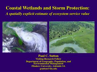
Coastal Wetlands and Storm Protection:A spatially explicit estimate of ecosystem service value Paul C. Sutton Visiting Research Fellow Department of Geography, Population, and Environmental Management Flinders University, Adelaide SA psutton@du.edu
Collaborators & Co-conspirators Robert Costanza Gund Institute of Ecological Economics, Rubenstein School of Environment and Natural Resources, University of Vermont, Burlington, VT 05405-1708, USA Octavio Pérez-Maqueo & M. Luisa Martinez Instituto de Ecología A.C., km 2.5 antigua carretera a Coatepec no. 351, Congregación El Haya, Xalapa, Ver. 91070, México. Sharolyn J. Anderson Department of Geography, University of Denver, Denver, CO, 80208, USA Kenneth Mulder W. K. Kellogg Biological Station, Michigan State University, Hickory Corners, MI 49060, USA How many e-mails? 100s easily How long? Over a year. We will meet at Stonehenge…
Ecosystem Services: What are they? • Ecosystem Services are the processes by which the natural environment produces resources useful to people, similar to economic services. Some Examples are: • The cycling of nutrients and energy • Provision of clean air and water • Pollination of crops • Pest and disease control • Climate regulation • Mitigation of natural hazards (what are we talking about?)
Ecosystem Services as ‘Public Goods’ • Ecosystem Services are often Public Goods in the economic sense in that they are non-rival in consumption (I can use a lighthouse to navigate my ship without impacting your ability to do the same), and non-excludable (in that if I owned the light house it would be difficult to provide the service only to those who paid for it). • Public Goods are a recognized ‘Market Failure’ in that both building lighthouses and providing many ecosystem services are really not good ideas for private enterprise despite the fact that Lighthouses and many Ecosystems have costs of production and/or maintenance that are greatly exceeded by the value of the services they provide. (e.g. Benefits exceed Costs)
Valuation of Ecosystem Services:Putting a dollar value on a ‘non-market’ service • Because Ecosystem Services are often destroyed or diminished by human action it behooves us to make reasonable estimates of their economic value to inform policy decisions regarding their fate. • Attempts at putting a dollar value on ecosystem services range from ‘squidgy’ contingent valuation studies (e.g. How much would you pay for the continued existence of [name your charismatic mega-fauna]? … To … • Rigorous and precise estimates of tangible values based on hard empirical evidence as presented here .
‘Geography’ or ‘Why Space Matters?’:Spatially Explicit Valuation of Ecosystem Services • Forests and other vegetated landcover provide an ecosystem service in the form of soil retention, or, mitigation of soil erosion. (that is reduced by fire) • Q1: How might ‘where’ this service is provided influence the ‘value’ of the service provided? • Q2: How might ‘the size of the burned patch’ influence the ‘value’ of the service provided? Before and After photos northeast of Sage Ranch, Topanga Fire, California
‘Coastal wetlands reduce the damaging effects of hurricanes on coastal communities by absorbing storm energy in ways that neither solid land nor open water can.’ *(Simpson and Riehl 1981). • What is the dollar value of the ‘reduced damage’? • What DATA does one need to answer this question? * Simpson, R.H. and Riehl, H. 1981. The hurricane and its impact. Louisiana State University Press, Baton Rouge, LA.
The Data Story… • 1) Table of all Hurricanes that hit the U.S. since 1980 w/ Name, Year, $ Damage, # Dead, etc. ... • 2) Shapefile of all the Hurricane Tracks since 1980 with windspeed, Category, Pressure, Temp • 3) Population and Nighttime Imagery to obtain ‘people in swath’ and ‘GDP in swath’ (modeled) • 4) LandCover (~30 Meter resolution - NLCD) to obtain ‘Wetlands’ information
The Damage Table (N = 34 Hurricanes) Data Source: www.em-dat.net/index.htm
The Storm Tracks (N = ~100) The Flying Spaghetti Monster The image above gives one an idea of what the tracks of the Atlantic hurricanes look like when displayed In a Geographic Information System. These are represented as lines and had to be buffered to a width That reasonably approximates the damaging swath of a hurricane. We chose a swath width of 100km. (Data Source: www.grid.unep.ch/data/gnv199.php Note: Each Storm Track consists of smaller sections Which have Category, Windspeed, Temp & Pressure Attributes
Buffer Existing Storms to 100 km (50 km per side) and Match to Damage Table (N=34) Andrew is an interesting example hurricane in that is represents one of the problems associated with this Analysis. Andrew did most of its damage during its first landfall in Florida. However, it went into the gulf of Mexico and struck the gulf coast later in its path. This multiple landfall issue raises some questions with Respect to our analysis. We believe we have to separate the two landfalls and the other data associatedWith the hurricane (damage, fatalities, GDP in swath, maximum wind speed, category, etc.).
Fleshing out the Table: 1) Population in Swath This image depicts the swath of Hurricane Hugo (1989) as it hit South Carolina. The shaded pink area is the population density (from LandScan2000) masked to only those areas within 100 km Of the coast. The zone of intersection of the swath of the hurricane and the population density on the coast is roughly demarcated by the green polygon. Sadly, these numbers have to be determined one at a time because The swaths of hurricanes often overlap – so, in essence we obeyed the instructions on the shampoo bottle: “Lather, Rinse, Repeat” (GIS is FUN )
Fleshing out the Table: 2) GDP in Swath This image shows a similar kind of intersection analysis for Hurricane Hugo except instead of population density The underlying coastal data is an estimate of the year 2000 GDP mapped at 1 km2 spatial Resolution. This model is derived from allocating the aggregate GDP of the United States to the individual pixels of this image on a linear basis in which the image is a nighttime satellite image composite derived from the DMSP OLS. So in this case the Estimate of GDP impacted by Hugo in 1989 was almost 1.7 billion dollars. Again, “Lather, Rinse, Repeat” for the rest of the hurricanes to produce a 2nd column in our table
Fleshing out the table: 3) Wetlands in Swath The image above shows both Woody Wetlands and Herbaceous Wetlands from the National Land Cover Database that was derived primarily from Landsat imagery. It Is at 30 meter resolution. The woody wets have to be processed separately from the Herbaceous wets in the same lather, rinse, repeat manner; however, we were getting Tired of making these images of Hurricane Hugo. In any case Hurricane Hugo passed Over 335 square kilometers of Herbaceous Wetlands and 2,306 km2 of Woody Wetlands. This image raises another question of how to assess the mitigating influence of wetlands when one takes into account the direction of the hurricane. Do the Woody Wets behind Charleston Really provide as much protection as the herbaceous wetlands in ‘front’ of Charleston. A question To ponder…… NLCD Data Reference: Vogelmann, J. E. and Howard S. M. 2001. Completion of the 1990's National Land Cover Dataset for the conterminous United States from Landsat Thematic Mapper Data and Ancillary Data Sources. Photogrammetric Engineering and Remote Sensing 64: 45-57.
This Tablewas builtwith the followingkey columns:TD/GDPHerb WetsWindSpeedto provide theRegression info
Regression Analysis ln (TDi /GDPi)= a + b1 ln(gi) + b2 ln(wi) + uiTDi = total damages from storm i (in constant 2004 $US);GDPi = Gross Domestic Product in the swath of storm i (in constant 2004 $US). The swath was considered to be 100 km wide by 100 km inland.gi = maximum wind speed of storm i (in m/sec)wi = area of herbaceous wetlands in the storm swath (in ha). ui = error Regression Parameters R2 = 0.60 Q: Why use TD/GDP For the dependant Variable? Observed vs. predicted relative damages (TD/GDP) for each of the hurricanes used in the analysis.
The Aggregate Conclusion • Mean Value of Coastal wetlands for storm protection: $33,000/ha/year • Coastal wetlands in the U.S. were estimated to currently provide $23 Billion/yr in storm protection services. Q: Average Annual Damage from Hurricanes in the U.S. from 1980 to present is roughly ~$4.3 Billion per year. How Can wetlands provide ~$23 Billion per year in protection?
Going Spatially Explicit:How does spatial context influence valuation? • Two approaches, two scales: States and Pixels • The State based approach: • Hurricane frequency per state with associated data • Mean Value ~$37,000 per hectare per year • The Pixel Based approach(at 1 km2 resolution): • Spatial context of nearby wetlands • Spatial context of nearby GDP • Frequency of Hurricanes (by category) at the pixel • Mean Value ~$ 31,000 per hectare per year The Math gets wild – Don’t ask me about it.
State Level Analysis • Data for each of the 19 states in the US that have been hit by a hurricane since 1980 (267 total hits) were used by Blake et al. (2005) to calculate the historical frequency of hurricane strikes by storm category. We calculated the average GDP and wetland area in an average swath through each state using our GIS database. We then calculated the annual expected marginal value (MV) for an average hurricane swath in each state using the following variation of the aforementioned regression equation: where: S = state sw = average swath in state s gc = average wind speed of hurricane of category c pc,s = the probability of a hurricane of category c striking state s in a given year GDPsw = the GDP in state s in the average hurricane swath wsw = the wetland area in state s in the average hurricane swath
Calculating Total Annual Value We then estimated total annual value of wetlands for storm protection as the integral of the marginal values over all wetland areas (the “consumer surplus) from the first or “marginal” hectare in the swath down to a value k, as: The above Equation estimates the avoided damages for each hurricane category in an average swath and multiplies by the probability of a given storm striking a state in a year. Value is thus only ascribed to wetlands that are expected to be in the swath of a hurricane. Residual analysis of our regression results suggested that our model over-predicted the damage mitigation for smaller wetland areas, so we only integrated MV down to k = 10,000 ha. This yields a conservative estimate of total damage avoided or total value.
Average Annual Value per Hectare of wetland per state as:AVstate = TVstate / Wetlandstate
Pixel Level Analysis Metamathemagical manipulations produce the equation below: “I came to Casablanca for the waters” “There is no water in Casablanca” “I was told there would be no math involved” “There is math involved.” “I was misinformed”. MVpxl is damage avoided ‘by the wetlands in that pixel’ e is 2.71828… α, β1, and β2 are the regression parameters, k=1000 gc is the average windspeed of category ‘c’ hurricanes wpxl is the area of wetlands within 50 km of the pixel GDPpxl is the GDP within 50 km of the pixel Pc is frequency of hurricane of category c at that pixel c varies from 1 to 5 (the categories of the hurricane) Avg windspeeds (meters/ sec): 77 (cat 5), 65(cat 4), 53(cat 3) , 45 (cat 2), 36 (cat 1)
Deconstructing the Valuation Equationand clarifying the ‘spatial explicitness’ Hurricane Frequency, GDP in Swath, and Wetlands in Swath all vary spatially thus we have a spatially explicit valuation method.
The ArcGIS ‘FocalSum’ Function:How we get the ‘GDP in Swath’ and ‘Wetlands in Swath’ values Focalsum( ): for each cell location on an input grid, adds the values within a specified neighborhood and sends the sum to the corresponding cell location on the output grid. We used it on both the GDP dataset and the wetlands dataset. Similar ‘Focal Function’ exist for mean, max, min, etc.
Creating the Hurricane Frequency Dataset At the pixel level, count the number of hurricanes that hit you for each category of storm (storms change category in space and time), five datasets (one for each category) smooth with a mean filter (focal mean)
A Single Pixel’s Value Calculation To the right is a Representation of a single pixel in the Mississippi Delta. It’s value is calculated below: NOTE: BUT THIS IS WRONG Frequency Data Whacked… Equations below are also incomplete.
Once We get Frequency Maps… We can make maps of Storm protection service Value from wetlands that Is truly spatially explicit. Just like the one to the Right but based on using Appropriately developed Frequency maps that Account for the spatial And temporal variation of Category (e.g. windspeed) Of storms through their Course…….
Discussion • Where is the ‘maximum wind speed’? • What about Woody Wetlands? • What about spatial orientation of wetlands with respect to Economic Activity? • What about multiple landfalls?
Conclusions • Coastal wetlands provide storm protection as an ecosystem service on the order magnitude of 10’s of BILLIONS of dollars per year in the U.S. alone. • A single hectare of wetlands provides a variable amount of services depending upon its spatial context with respect to GDP in space, other wetlands in space, and the frequency with which it is hit by hurricanes of various categories. Values range from 10s of dollars to Millions of dollars per hectare.