Download

1 / 23
230 likes | 402 Views
The use of the Chi-square test when observations are dependent by Austina S S Clark University of Otago, New Zealand. Outline of the talk. Motivation Introduction Methodology Example Simulation. Introduction

E N D
The use of the Chi-square test when observations are dependentby Austina S S ClarkUniversity of Otago, New Zealand
Outline of the talk • Motivation • Introduction • Methodology • Example • Simulation
Introduction When the Chi-square test is applied to test the association between two binomial distributions, we usually assume that cell observations are independent. If some of the cells are dependent we would like to investigate: 1. how to implement the Chi-square test and 2. how to find the test statistics and the associated degrees of freedom.
We will use an example of influenza symptoms of two groups of patients to illustrate this method. One group of patients suffered from H1N1 influenza 09 and the other from seasonal influenza. There were twelve symptoms collected for each patient and these symptoms were not totally independent.
Methods • We review the medical records of all sixty four adult patients (18 years old) with a laboratory confirmed diagnosis of two types of influenza, namely seasonal influenza (F) and H1N1 influenza 09 (S), between 17 June and 31 July, 2009 in an Australian hospital. • Twelve symptoms were extracted from each patient’s records using 0 for no symptom and 1 for the symptom. • Some of the symptoms are not independent.
We examined the correlation matrices for the two groups of patients, F (seasonal influenza) and S (H1N1 09). • If the correlation was significant then we calculated the two covariance matrices respectively and then pooled them together to form a pooled covariance matrix • Next we found out the mean proportion of symptoms for each of the symptoms, say p. • and .
In order to find the true proportion difference between the two groups we need to find the difference between and . Since there is correlation between the p variables we can not use the Penrose distance (Manly B F J, 1994). However, we have instead two alternatives to incorporate the correlation. Firstly we apply the Mahalanobis distance, , (Manly, 1994), which takes into account the correlations between variables, where
can be thought of as a multivariate difference for the two observations and , taking account of all p variables. We assume that the populations which and come from are multivariate normally distributed - then the values of will follow a chi-square distribution with p degrees of freedom. Alternatively we may apply the method suggested by Greenhouse S W and Geisser S (1959) by transforming .
Let then , where are not independent. Now let . The values of follows a chi-square distribution , where is a multiplier and can be approximated (Satterthwaite F E, 1941, 1946).
Next we find the eigenvectors, , and eigenvalues, , of the covariance matrix . Let , then , where are independent. Next let and
This indicates that the values of also follows the chi-square distribution . The properties of the expected value and variance of and can be used to find values of and . It can be deduced that where are the eigenvalues of .
We also find that This follows that and
Example • As mentioned early, we review the medical records of sixty four adult patients with a laboratory confirmed diagnosis of two types of influenza. • Of these 64 patients,16 had seasonal influenza (F) and 48 had H1N1 09(S). • All patients were admitted between 17 June and 31 July, 2009 in an Australian hospital. • The aim here is to compare the twelve clinical symptoms presented by these two groups of patients.
These 12 symptoms are listed below: • S1: coryza • S2: fever • S3: cough • S4: breathlessness • S5: chest pain • S6: sore throat • S7: lethargy • S8: myalgia • S9: vomiting • S10: diarrhoea • S11: abdominal pain • S12: other gastro-intestine upset
Since these symptoms are not totally independent, we will use the methods mentioned above. The results are: Method 1: = 0.9384, which follows a distribution with p-value= 0.9999. Method 2: = 0.1215, which follows a distribution with =0.2873, =7.2596 and p-value= 0.9997.
Results • Both methods showed that there is no significant difference of the twelve symptoms between the two types of influenza. • Patients with H1N109 (S) were significantly younger than patients with seasonal influenza (F), vs with p-value < 0.01. • The mean duration of symptoms prior to presentation was 4 days, with fever, cough and dyspnoea being the most common symptoms in both groups. • Pneumonia occurred in 44% and 38% of H1N1 09 and seasonal influenza patients respectively.
This study shows that the H1N1 09 influenza virus causes clinical disease in humans comparable to the seasonal influenza strains in this Australian city during the period 17 June to 31 July, 2009 . Conclusion
Simulation • We used MATLAB and simulated 200,000 times of the proportions of the twelve symptoms (for both methods) for the two groups of influenza respectively. • The results are shown below.
References • Greenhouse S. W. and Geisser S. (1959). On methods in the analysis of profile data. Psychometrika, 24, 95-112. • Huynh H. and Feldt L.S. (1976). Estimation of the Box correction for degree of freedom from sample data in randomized block and split plot designs. JEBS, 1, 69-82. • Manly B. F. J. (1994). Multivariate statistical Methods. A Primer. Chapman & Hall. • Satterthwaite F.E. (1946). An approximate distribution of estimates of variance components. Biometrics bulletin, 2, 110-114.