Download
1 / 61
720 likes | 1.07k Views
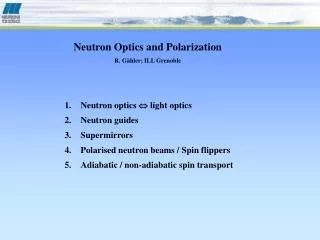
Neutron Optics and Polarization R. G ähler; ILL Grenoble. Neutron optics light optics Neutron guides Supermirrors Polarised neutron beams / Spin flippers Adiabatic / non-adiabatic spin transport. Neutron optics light optics.

E N D
Neutron Optics and Polarization R. Gähler; ILL Grenoble • Neutron optics light optics • Neutron guides • Supermirrors • Polarised neutron beams / Spin flippers • Adiabatic / non-adiabatic spin transport
Neutron optics light optics scalar matter waves transversal e.m. waves (diffraction in time) fermions bosons (beam correlations) k2 k (index of refraction)
The wave equations for light and matter waves in vacuum: General case: Stationary case: light waves: Helmholtz equ. matter waves: Schrödinger equ. E ; same patterns; Light waves: periodic , propagating with c; matter waves: similar to diffusion equationexcept for ‘i’ Optics in space: Same physics; Optics in time: Different physics;
r r What is special with optics in time for matter waves? The Green’s function in the stationary case:(propagation of a -like excitation in space) for : Spherical waves The Green’s function in the non-stationary case:(propagation of a -like excitation in space and time) for : at fixed time : at fixed position r: A broad spectrum is emitted; The higher the frequency, the faster the propagation; Can be expanded to a plane wavefor a short period in time and space; t
t k0; 0 r opening time 2T Example: diffraction of matter waves from a ‘slit in time’ scattered wave at opening of slit Incoming wave at opening of slit
Example: diffraction of matter waves from a ‘slit in time’ Evaluate the exponent: Minimum for the exponent: exponent of integrand classical time of propagation the phase is stationary around 0 Diffraction in Time Significant contributions to the amplitude may only be accumulatedduring time periods when the phase is constant: Thus the integral may only be evaluated around its extremum. ‘Method of stationary phase’ 2nd order expansion leads to Fresnel integrals in time, analogue to diffraction in space.
Plane of detection Lateral beam correlations of an extended source of matter waves / e.m. waves Can we measure a diffraction pattern from two slits(separation xc)? (for simplicity we consider only one wavelength) xc extended incoherent sourcee.g. sun; moderator of reactor; light bulb Because of incoherence, we sum the intensities of all individual waves but not add the amplitudes before quadrature.‘Each wave interferes only with itself.’
Plane of detection Slightly displace all wave fronts in direction of propagation, so that they are in phase at the two slits. This does not influence the diffraction pattern, as only the phase difference at both slits is relevant. If all waves are fairly well in phase at both slits, then one measures a pattern with high contrast. xc For this distance xc, the contrast of the diffraction pattern will be okay. The wave field is coherent over the distance xc, though in reality the waves are not in phase. xc is called the ‘lateral coherence length’ of the field. This construction is possible anywhere in the wave field! With this construction, the wave field resemblesthe pacific ocean
xc L 2a From simple geometry: xc = L / ka; k = 2/; This holds for matter waves and light waves! xc 100Å for a neutron beam; xc 1m for stars (Michelson);
Longitudinal coherence of a ‘quasi-stationary’ non-monochromatic beam Can we measure a diffraction pattern (double slit in time) from one slit, which is at one position at two different times, which are separated by tc? This slit is here at t0, then it disappears and is only back here at t0 + tc Point like sources may emit spherical waves of different wavelengths at arbitrary times
Slightly displace all wave fronts in time (here in direction of propagation), so that they are in phase at the time t0, when the slit is there. This does not influence the diffraction pattern, as only the phase difference at both times is relevant. We will only be able to measure the double slit in time, if during the time interval t0 to t0+tc the accumulated phases of all waves will be fairly the same, say within = 1 Coherence length lc = 2/ You may construct this coherence length (wave packet) at any time and any position along the beam. It remains constant. The product xc yc lc is the coherence volume Vc
Difference matter waves – light waves, concerning coherence • quantitative: N0, the number of particles / coherence volume: • N0 = 10-15 at neutron sources; N0 = 10-1at X-ray sources; • qualitative: 2 fermions should not be in one coherence volume; • The Hanbury-Brown / Twiss experiment gives anti-correlations for neutrons, but correlations for light; If, by chance, most waves are in phase at slit A a during the coherence time, then there is a high probability to measurea particle behind A.Then, if distance AB is smaller than the lateral coherence length, the waves willalso be in phase at B and then the probability to measure a second particlebehind B is high as well. A Det. Correlated det. B Det.
Another difference light optics neutron optics light: c = /k neutrons: v = k /m In general, the index n of diffraction is defined as n = k’/k; A) Light entering a slab of matter: c’ < c k’ > k n > 1; B) Neutrons entering a slab of matter: For most materials the potential V is positiv. v’ < v k’ < k n < 1;
2. Neutron guides 12 guides from one beam tube at ILL
Analytic calculation of neutron guides Potential step V0 for of a material surface : N : number density of atoms bc : coherent scattering length of the atoms no Bragg scattering; absorption negligible; In case of different atoms i, the weighted average <N·bc>i has to be taken. For positive values of bc, which holds for most isotopes, V0 is positive (n<1), thus neutrons are totally reflected, if their kinetic energy Ekin perpendicular to the surface is smaller than V0. Ekin = ½mv2 = 2k2/(2m) < V0 (mv = k = h/; k is the vertical wavevector and the corresponding vertical wavelength)
The critical angle of reflection c : k k c Potential ½mv2 = 2k2/(2m) < V0 k = (4 N bc)½ k is the vertical wavevector This defines a critical angle of total reflection c k / k = (4 N bc)½ / k = (N bc/ )½ k [Ni] = 1.07 ·10-2 Å-1 m=1; (most guides H1/H2) Supermirrors of n-guides typically have m =2 k [SM:m=2] = 2.14 ·10-2 Å-1; Rule of thumb: For Ni, the critical angle c[degrees] 0.1 wavelength [Å];
Basic properties of ideal bent guides I All refections are assumed to be specular with reflectivity 1 up to a well defined critical angle c and with reflectivity 0 above c . z a The reflection angle at the outer wall a is always bigger than at the inner wall i . x a coordinate system rotates with guide axis i -a a- i
Basic properties of ideal bent guides II • There are two types of reflections: • Zig-zag reflections (large a) • Garland reflections (never touching the inner wall) (small a) • If the max. reflection angle allows only Garland reflections near the outer wall, then the guide is badly filled. • If high a i the filling of the guide will be fairly isotropic. a i transition from Garland- to Zig zag reflections
Basic properties of ideal bent guides III a After at least one reflection of all neutrons*, the angular distribution in the guide is well defined. The angles always repeat. *after the direct line of sight transition from Garland- to Zig zag reflections
Basic properties of bent guides IV At each point in the long guide, the angular distribution is symmetric to the actual guide axis, as there exists always a symmetric path which is valid. This holds of course also for the guide exit. a For a given a, the angular width 2 nearthe outside is larger than near the inside; a a The differential flux d /d is constant all across the guide (Liouville!), however the maximum angular width 2 is different. This width is proportional to the total intensity at each point. (for = const.) We have to calculate to get the intensity!
The Maier-Leibnitz guide formula a x x1 x2 - a a- y 90-a y = ·sin(a- ) ·(a- ); x1 = - ·cos(a- ) /2 ·(a- )2; x2 = y ·tan y· (a- ) ; x = x1 + x2 = /2 ·(a2- 2); 2 = a2 - 2x/; a
The Maier-Leibnitz guide formula a x x1 x2 - a a- y y = ·sin(a- ) ·(a- ); x1 = - ·cos(a- ) /2 ·(a- )2; x2 = y ·sin y· (a- ) ; x = x1 + x2 = /2 ·(a2- 2); 2 = a2 - 2x/; a
The Maier-Leibnitz guide formula a x x1 x2 - a a- y y = ·sin(a- ) ·(a- ); x1 = - ·cos(a- ) /2 ·(a- )2; x2 = y ·sin y· (a- ) ; x = x1 + x2 = /2 ·(a2- 2); 2 = a2 - 2x/; a
The intensity distribution in a long curved guide as function of To calcukate the max. transmitted divergence, we choose: a = c = k/ k; Plot of = (c2 - 2x/)½ as function of x for different c as parameter: For = c the inner wall just does not get touched. In this case the divergence is 0 at the inner wall. The wavelength , corresponding to this c is called characteristic wavelength *. c2 > 2a/ c2 = 2a/ parabolas open to the left c2 < 2a/ 0 a x width of guide
The critical parameters of a long curved guide * = (2a/)½; * = characteristic angle; With * = k / k* we get: k* = k(2a/)-½; k* = characteristic k-vector; With * = 2 / k* we get:* = 2 (2a/)½ / k;* = characteristic wavelength; F[ = (c2 - 2x/)½/ = c ] Filling factor F (intensity ratio curved guide/straight guide): c = 2* c F = 0.93 a* = a for c *; a* = c2/2 for c *; c c = * F = 2/3 c F = 1/6 c =½ * 0 a x a/4 F(c= 2*) = 0.93; F(c= */2) = 1/6; F(c= *) = 2/3;
Changes from m=1 m=2 and from a 1.5a Replacing a Ni guide (m=1) by a SM guide (m=2) doubles k and c. Increasing the guide width from a 1.5a increases * by 1.5½and also increases the direct line of sight [Ld = (8a)½] by1.5½. New critical angle c from increase of m For * the intensity increases by a factor 4. new 2c c old New characteristic * from increase of width c/2 0 a 1.5a a/4 x For * the intensity increases by more than a factor 4 from doubling of c. [c/2 c is shown.]
Changes in parameters along a guide: From here on the final angular distribution is well defined. a) b) Bad example: Two successive guide sections of the same *: * */m; a) low m; low * b) high m; high * Outgoing beam of high divergence;loss in phase space density!!
Changes in parameters along a guide: Example: Split a guide (width a) into two guides (width a/2), reduce radius of curvature to /2 and keep c2 constant = [c2 - 2x/]½ = c [1 - 2x/(c2)]½ The dashed line shows the angular distribution in the original guide The full lines show the max. possible angular distribution in the split guides All neutrons will be transmitted. Loss in phase space density? c2 = 2a/ = * 0 x a Both curves intersect at a, because c2 is constant a/2 a/2
Estimate of main n-guide losses Reflectivity: Garland refl.: lg = 2 ; Zig-zag refl.: lz = (a - i ); or lz d/; Rn = (1 - )n 1 - n ; for << 1; for R = 0.97 and L = 1.2 L0; n 3 ( = 2700m; = 1/200) beam transmission fR by reflectivity R: < fR > = 0.9; higher for long SM-guides! l = mean length for one reflection from side walls; n = mean number of reflections; R = reflectivity; L0 = length of free sight; L=100m Alignment errors: Gauss distrib.: f(h) = exp(-h2/hf2) / (-1/2 hf ) Transmission fa = 1 - L/Lp hf -1/2/a; For L = 1.2 L0 ; a = 3 cm, Lp = 1m, L = 100m and hf = 20 m: mean transmission due to alignment errors: fa = 0.96; For guide of 20x3 cm, the necessary precision on top / bottom is 7 times worse (0.14 mm). hf = mean alignment error; a = guide width (30 mm); Lp = length of plates; h
Estimate of main n-guide losses waviness: Let the neutron be reflected under angle + instead of . For 6 reflections, L = 1.2 L0 ; k = 0.7k*: fw = 1 - w /*; For w = 10-4, * = 1.7 10-3 [1Å, Ni]: fw = 0.94; The outer areas of the intensity distribution I() are more affected than the inner ones. fw : transmission due to waviness; w = RMS waviness; * = characteristic angle of guide I() without waviness with waviness c w = 2·10-4 for the new guides seems acceptable (m=2!) The angle between the guide sections can be treated as waviness. = 1/27000 for H2.
Flux d/d for given source brilliance d2/dd and distance z from source: Flux d/d in long straight guide for constant source brilliance d2/ddif angular acceptance in guide x y is smaller than angular emittance of source: Summary of main guide formulas = radius of curvature a = width of guide x = width from outer surface k =max. vertical wavevector; = angular width w.r.t. guide axisc k / k = (4 N b)½ / k = (N b/ )½ k [Ni] = 1.07 ·10-2 Å-1 m=1; k = 1.07 ·x · 10-2 Å-1; [SM: m=x] Supermirrors of n-guides typically have m =2 k [glass] = 0.63 ·10-2 Å-1; k [Ni-58] = 1.27 ·10-2 Å-1; = (c2 - 2x/)½; = angular width at output of curved guide; c = critical angle of total reflection; * = (2a/)½; * = characteristic angle; conditions: each neutron is at least once reflected at outer surface and reflectivity is step function up to c; * = 2 (2a/)½ / k;* = characteristic wavelength;
Loss V in intensity due to gap of length L for a guide of cross scection ab: a* = a for c *; a* = c2/2 for c *; F = filling factor of guide Summary of main guide formulas L02= 8a; L0 = direct line of sight of bent guide; = a-(L0/2-dL)2/2R; = width of direct sight of bent guide; dL = missing length to L0 xb= L2/(2); xb = lateral deviation from start direction; L = length of guide; ng = L/(2 ) ; nz = L/( (a - i )); or nz L /a;n = number of reflections; ng for Garland; nz for Zig-zag refl.; fw = 1 - w /*; fw = loss due to waviness; w = RMS value of waviness; L = 1.2 ld ; fa = 1 - L/Lp hf -1/2/a; fa = loss due to steps; hf = RMS value of alignment error;
3. Supermirrors (polarising) A rule of thumb to estimate reflectivity and number of layers* • for calculations see e.g.: • F. Mezei; Commun.Phys.1(1976)81; + Corrigen. : Commun.Phys.2(1977)41; (first paper) • J. Hayter, A Mook: J. Appl. Cryst.: 22(1989)35; (used for supermirror production)
Mirror reflection on multilayer in 1D magnetic layers b2 = bc2 bm; Plane wave; k0 non-magn. layers: b1 = bc1 bc2 + bm For spin : bc2 + bm bc1 bc2 bc1 For spin : bc2 – bm bc1; bc1 0 bc2 - bm bc1
Reflectivity of multilayer in 1D Plane wave; 0 magnetic layers n2 = nc2 nm 1 + 2nm; d 0 non-magn. layers: n1 = nc1 1 Jump in phase at reflection; Reflectivity at normal incidence at one layer (far beyond total refl.): = 0 for reflecting on smaller n; = for reflecting on higher n; Raleigh formulas • For the proper 0 =2d the reflected waves fromall boundaries are in phase R (2nm)2 R (2Z2nm)2 for reflection at Z double layers of width d;
Reflectivity of multilayer in 1D Estimate of number of double layers Z for reflectivity near 1: R (2Z2nm)2 for reflection at Z double layers of width d; With nm = bmZ2/2 = 2: (However, 1. Born approx. is very bad here!Because of attenuation less layers are needed) For R 1: Z 1/(4 2); Estimate of the reflected -band: The phase variation of the reflected waves from all 2Z boundaries should be: /2; Reflected wavelength band 1/Z 2 ; Phase variations from micro roughness of given r : 1/ It is very hard to make good high –m supermirors!
Co/Ti polarising supermirrors; K. Andersen, ILL q B substrate Nb Nb substrate B B N(+p) No qc ! Nb N(-p) No magnetic field
Fe/Si polarising supermirrors; K. Andersen, ILL q Nb Nb Nb B No qc ! N(+p) N(-p) l=3Å : labs = 70cm Si substrate
concept of neutron supermirrors; Swiss Neutronics neutron reflection at grazing incidence (< ≈2°) @ smooth surfaces @ multilayer @ supermirror • refractive index n < 1 • total external reflection e.g. Niqc = 0.1 °/Å
concept of neutron supermirrors; Swiss Neutronics • the m – value • range of supermirror reflectivity in units ofqc, nat. Ni • layer sequence of Hayter & Mook1 • l/4 layer thickness • overlapp of superlattice Bragg peaks regime of total reflection regime of supermirror 1J. B. Hayter, H. A. Mook, Discrete Thin-Film Multilayer Design for X-Ray and Neutron Supermirrors, J. Appl. Cryst. 22 (1989) 35
concept of neutron supermirrors; Swiss Neutronics K. Soyama et al., NIMA. 529 (2004) 73 layer material – contrast of SLD (r · b) • reflectivity • bNi = 10.3 fm • bTi = -3.4 fm • Ni/Ti supermirrors • General goals: • high m - value • high neutron reflectivity • large number of layers, e.g.m = 2 120 layers (R 90%)m = 3 400 layers (R 80%) m = 4 1200 layers (R ≈ 75%)m = 5 2400 layers (R ≈ 63%) • interface quality • internal stress M. Hino et al., NIMA. 529 (2004) 54
Ni/Ti supermirrors – reactive sputtering NiNx reactive sputtering of Ni in Ar:N2 atmosphere Limit for stability • increase of reflectivity withincreasing content of N2during sputtering of Ni layers • increase of internal strain damage of glass substrate
Ni/Ti supermirrors – high ‘m’ ; Swiss Neutronics m = 3 m = 4 reflectivity simulation:SimulReflec V1.60, F. Ott, http://www-llb.cea.fr/prism/programs/simulreflec/simulreflec.html, 2005
polarizing supermirrors – ‘remanent’ option concept of ‘remanent’ polarizing supermirrors • magnetic anisotropy • high remanence • guide field to maintain neutron polarization ≈ 10 G • switching of polarizer/analyzer magnetization short field pulse ≈ 300 G
4. Polarised neutron beams / spin flippers Emag = n B = 610-8 eV/Tesla; For thermal/cold neutrons: Emag Ekin: the neutron trajectory is hardly affected by the magnetic interactions;the spins can easily be turned but not easily be pushed or pulled; (longitudinal and lateral Stern Gerlach effects are small effects); = /S; = gyromagnetic ratio;
Graphical interpretation of • dS B; precession around B; • dS S; precession frequency is constant; • In both cases: dS Ssin; • during dt, the angular change of Ssin around B is constant: • the precession ‘Larmor’ frequency L does not depend on ; B B Ssin2 Ssin1 dS1 dS2 S 1 S 2 dS1 dS2 L = 2B; = 2.9 kHz / G A neutron entering a static B-field, precesses with L around the B-field;
QM -description of a neutron beam, entering a B-field Plane wave, entering a static B-field ? x B = Bz y y = 0 Neutrons: s = ½; µ 0; 2 states + and - with different kinetic energies E0 µB Static case [dB/dt = 0]: no change in total energy ( = 0) but change in k; µB Ekin v is the classical neutron velocity;
Both states have equal amplitudes, as the initial polarization is perpendicular to the axis of quantization (z-axis); These amplitudes are set to 1 here. 1 1 = 0 Energy diagram: Ekin [-Epot] += 0ei k y E0 2µB k = µ B/v -= 0e –i k y y y=0