Download

1 / 46
470 likes | 667 Views
Automatic Segmentation of Pulmonary Nodules in Computed Tomography Images. Given by Timothy R. Tuinstra Cedarville University At the IEEE-Dayton Section Computer Society Meeting. 3.17.09. Background. Lung cancer is the leading cause of cancer death in the U.S. 215,000 new cases in 2008.

E N D
Automatic Segmentation of Pulmonary Nodules in Computed Tomography Images Given by Timothy R. Tuinstra Cedarville University At the IEEE-Dayton Section Computer Society Meeting 3.17.09
Background • Lung cancer is the leading cause of cancer death in the U.S. • 215,000 new cases in 2008. • About 160,000 people died of lung cancer in the U.S. alone in 2008. • Computer aided detection and diagnosis (CADD) tools are critical to the fight.
What Do Lung Nodules Look Like? Lung Nodule
Research Goals • To develop a robust automatic segmentation algorithm for pulmonary nodules that compares well with radiologist segmented data.
Image Thresholding High Threshold Low Threshold One of the main difficulties with segmentation here is that extraneous structures exhibit similar intensities.
Morphological Processing: Connected Components Pixels are said to be “connected” to a given pixel if they are one of the neighbors (4 or 8) of the pixel. Connected component analysis will preserve only thresholded pixels that are connected to the cue point. Before Connected Components After Connected Components
Morphological Processing:Opening Small Radius: Large Radius: Resulting Segmentation: Resulting Segmentation:
Morphological Processing:Opening Before Opening After Opening Note the broken link
One more connected Component Analysis Before Connected Components After Connected Components
Segmentation Engine Input VOI Output Segmentation Threshold Connectivity Requirement Morphological Processing Connectivity Requirement R T T - Intensity Threshold R – Structuring Element radius LIVE DEMO!
Big Ideas: • Create candidate segmentations • Predict the quality of the candidates and pick the best one • Can we automate this?
How good is a Segmentation? Overlap Measure: Truth Segmentation kth Candidate Segmentation
Volume of interest Structuring Element Radius Intensity Threshold Candidate Segmentation Feature Vector Predicted Overlap Prediction of Overlap Artificial Neural Network Segmentation Engine Extract Features
The Neural Network • We experimented with both multilayer perceptrons and radial basis function(RBF) networks to predict the overlap. • General regression radial basis function networks (GRNN) were chosen because of the speed of training and consistency of results. • GRNN networks are known for their ability to approximate functions. • GRNN networks use examples to respond to previously unseen inputs.
The Neural Network • Generalized Regression Radial Basis Function Network: maps kth feature vector jth “center” jth radial basis function jth weight
φ1 φ2 Σ φM The Network Architecture
Measured Segmentation Features Network Centers Network Weights Desired Network Outputs (Desired Overlap) Radial Basis Functions Gaussian Function Training the Network Select M training vectors together with corresponding desired outputs.
The Training Data • 72 nodules were from the Early Lung Cancer Action Program (ELCAP). • 1.25 mm slice spacing and thickness • 76 nodules were from the University of Texas Medical Branch (UTMB). • 2.5 and 5 mm slice spacing and thickness • These nodules were manually segmented using T & R method.
76 Nodules 72 Nodules SFS weights SFS weights SFS weights 76 Nodules The Training Data • The training data was partitioned into two sets: • One set was used to determine weights. • The second set was used to select features.
Feature Selection • Features were selected from a pool of 50 using Sequential Forward Selection (SFS). • SFS: • Train a network with each of the 50 features. • Select the one that provides the best mean overlap across the training set and include as winning feature #1. • Create networks using #1 and each one of the remaining features. • Find winner #2 and include in feature set. • Continue until adding additional features no longer helps.
Winning features • 1) Mean convergence index (MCI) • 2) Mean surface gradient • 3) Mean separation in the axial direction • 4) Radial Deviation
Estimate the 3-D gradient of the intensity volume of interest: Create a radial vector field: Divide these two vector fields by their magnitudes to find unit vector fields. Compute the inner product (scalar field): Mean Convergence Index
Candidate 1 Candidate 2 Resulting Scalar Field The Mean Convergence Index is the mean of the pixels contained in the candidate segmentation. Obviously, the green segmentation has a higher MCI than the red segmentation candidate.
Mean intensity in segmentation Mean intensity axial boundary voxels Other Features • Mean Surface Gradient: Number of voxels on the surface of the segmentation • Mean Intensity Separation in Axial Direction:
Other Features • Radial Deviation: Computed in the same way as MCI except only for boundary voxels.
Automatic Selection of T & R Output Segmentation Input VOI Threshold Connectivity Requirement Morphological Processing Connectivity Requirement Artificial Neural Network Feature Extractor Update T & R
Updating T & R • “Exhaustive” Search • Test candidates on a uniformly spaced grid of T & R and choose largest predicted overlap. • Simulated Annealing • Move through the T & R space in a purposeful manner “looking” for the largest predicted overlap. • Reduces computation time. • Golden Section Search • Apply across thresholds. • Reduces computation time.
Minimizing via simulated annealing • Choose an initial value for R & T • Compute predicted quality for this R & T: • Compute Segmentation • Compute Features • Use NN to compute cost • Take a random step in R & T space • Max step size based on previous cost • High quality yields small step (we must be close) • Low quality yields larger step
Minimizing via simulated annealing • At the new location, compute the segmentation and evaluate the predicted quality. • If it is less than the previous one…keep it. • If it is more…keep it with some small probability that gets smaller with # of iterations. This keeps us from getting stuck in local minima. • Repeat until some criteria is satisfied. • Always keep the highest quality output seen as the best R & T • Example trajectories are shown in the next few slides.
Minimizing via Golden Section Search • Apply this search along T for 4 different values for R. • Find the 4 minima. • Choose the smallest of these 4.
What data was used for segmentation testing? • Lung Imaging Database Consortium (LIDC) data • 69 Nodules • Manual segmentations of up to 4 radiologists are contained in the data. • Nodules with 3 or 4 radiologists segmentations were used. • Voxels considered to be part of the nodule by 3 or 4 radiologists comprise the truth mask to which we will compare.
Example Segmentation LIDC #34: Overlap = 81.5% Quality Function
Example Segmentation LIDC #36: Overlap = 40.6% Quality Function
Example SegmentationLIDC #41 Quality Function Overlap = 68.2%
Acknowledgments • Dr. Russell Hardie, University of Dayton • Ph.D. advisor and mentor • Dr. Steven Rogers, AFRL • Neural network expert