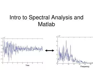
Introduction to Spectral Analysis and MATLAB: Quantifying Sound Tone Changes of a Race Car
420 likes | 533 Views
Learn how to quantify changes in a race car's tone as it passes you using Fourier Transform in MATLAB. Explore time and frequency domains, power spectral densities, and more in this practical guide.

Introduction to Spectral Analysis and MATLAB: Quantifying Sound Tone Changes of a Race Car
E N D
Presentation Transcript
Intro to Spectral Analysis and Matlab Q: How Could you quantify how much lower the tone of a race car is after it passes you compared to as it is coming towards you? How would you set the experiment up?
Running the Experiment . Data is often recorded in the time domain. The stored dataset is called a timeseries. It is a set of time and amplitude pairs.
Frequency Domain (Do a Fourier Transform on Timeseries) We have converted to the Frequency Domain. This dataset is called a Spectra. It is a set of frequency and Amplitude pairs.
What’s the Frequency? What’s the Period? What will this look like in the Frequency Domain? Time Domain
What’s the new (red) period? How Does its amplitude Compare to the 1 s signal?
Power Spectral Densities Secondary Microseism (~8 s) Primary Microseism (~ 16 s)
Sampling Frequency • Digital signals aren’t continuous • Sampled at discrete times • How often to sample? • Big effect on data volume
Aliasing FFT will give wrong frequency
Nyquist frequency • Can only accurately measure frequencies <1/2 of the sampling frequency • For example, if sampling frequency is 200 Hz, the highest theoretically measurable frequency is 100 Hz • How to deal with higher frequencies? • Filter before taking spectra
Summary • Infinite sine wave is spike in frequency domain • Can create arbitrary seismogram by adding up enough sine waves of differing amplitude, frequency and phase • Both time and frequency domains are complete representations • Can transform back and forth – FFT and iFFT • Must be careful about aliasing • Always sample at least 2X highest frequency of interest
To create arbitrary seismogram • Becomes integral in the limit • Fourier Transform • Computer: Fast Fourier Transform - FFT
Basin Thickness • Sediment site • 110 m/s /2.5 Hz = 44 m wavelength • Basin thickness = 11 m • Peat Bog • 80 m/s /1 Hz = 80 m • Basin thickness = 20 m
Station LKWY, Utah raw Filtered 2-19 Hz Filtered twice
Station LKWY, Utah raw Filtered 2-19 Hz Filtered twice