Understanding Spectral Analysis in Voiced Speech: A Comprehensive Overview
390 likes | 540 Views
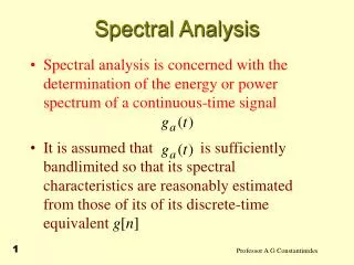
This lecture notes explore the spectral analysis of voiced speech sounds, focusing on the complex wave emitted from the glottis during voicing and how humans shape this spectrum to create distinct speech sounds. We examine Fourier's Theorem, the principles of Fourier Analysis, and the use of Discrete Fourier Transform (DFT) and Fast Fourier Transform (FFT) in speech analysis. Through analyzing spectrograms and the impact of different window types on the spectral analysis process, we clarify the relationship between complex waves and their sinewave components, providing insights into the acoustic analysis of speech.

Understanding Spectral Analysis in Voiced Speech: A Comprehensive Overview
E N D
Presentation Transcript
Spectral Analysis Bonus Lecture Notes!
The Source • The complex wave emitted from the glottis during voicing= • The source of all voiced speech sounds. • In speech (particularly in vowels), humans can shape this spectrum to make distinctive sounds. • Some harmonics may be emphasized... • Others may be diminished (damped) • Different spectral shapes may be formed by particular articulatory configurations. • ...but the process of spectral shaping requires the raw stuff of the source to work with.
Spectral Shaping Examples • Certain spectral shapes seem to have particular vowel qualities.
Spectrograms • A spectrogram represents: • Time on the x-axis • Frequency on the y-axis • Intensity on the z-axis
Ch-ch-ch-ch-changes • Check out some spectrograms of sinewaves which change frequency over time:
The Whole Thing • What happens when we put all three together? • This is an example of sinewave speech.
The Real Thing • Spectral change over time is the defining characteristic of speech sounds. • It is crucial to understand spectrographic representations for the acoustic analysis of speech.
Life’s Persistent Questions • How do we get from here: • To here? • Answer: Fourier Analysis
Fourier’s Theorem • Joseph Fourier (1768-1830) • French mathematician • Studied heat and periodic motion • His idea: • any complex periodic wave can be constructed out of a combination of different sinewaves. • The sinusoidal (sinewave) components of a complex periodic wave = harmonics
Fourier Analysis • Building up a complex wave from sinewave components is straightforward… • Breaking down a complex wave into its spectral shape is a little more complicated. • In our particular case, we will look at: • Discrete Fourier Transform (DFT) • Also: Fast Fourier Transform (FFT) is used often in speech analysis • Basically a more efficient, less accurate method of DFT for computers.
Spectral Slices • The first step in Fourier Analysis is to window the signal. • I.e., break it all up into a series of smaller, analyzable chunks. • This is important because the spectral qualities of the signal change over time. • Check out the typical window length in Praat. a “window”
The Basic Idea • For the complex wave extracted from each window... • Fourier Analysis determines the frequency and intensity of the sinewave components of that wave. • Do this about 1000 times a second, • turn the spectra on their sides, • and you get a spectrogram.
Possible Problems • What would happen if a waveform chunk was windowed like this? • Remember, the goal is to determine the frequency and intensity of the sinewave components which make up that slice of the complex wave.
The Usual Solution • The amplitude of the waveform at the edges of the window is normally reduced... • by transforming the complex wave with a smoothing function before spectral analysis. • Each function defines a particular window type. • For example: the “Hanning” Window
There are lots of different window types... • each with its own characteristic shape Hamming Bartlett Gaussian Hanning Welch Rectangular
Window Type Ramifications • Play around with the different window types in Praat.
Ideas • Once the waveform has been windowed, it can be boiled down into its component frequencies. • Basic strategy: • Determine whether the complex wave correlates with sine (and cosine!) waves of particular frequencies. • Correlation measure: “dot product” • = sum of the point-by-point products between waves. • Interesting fact: • Non-zero correlations only emerge between the complex wave and its harmonics! • (This is Fourier’s great insight.)
A Not-So-Complex Example • Let’s build up a complex wave from 8 samples of a 1 Hz sine wave and a 4 Hz cosine wave. • Note: our sample rate is 8 Hz. • 1 2 3 4 5 6 7 8 • A 1 Hz 0 .707 1 .707 0 -.707 -1 -.707 • B 4 Hz 1 -1 1 -1 1 -1 1 -1 • C Sum: 1 -.293 2 -.293 1 -1.707 0 -1.707 • Check out a visualization.
Correlations, part 1 • Let’s check the correlation between that wave and the 1 Hz sinewave component. • 1 2 3 4 5 6 7 8 • C Sum: 1 -.293 2 -.293 1 -1.707 0 -1.707 • A 1 Hz: 0 .707 1 .707 0 -.707 -1 -.707 • C*A Dot: 0 -.207 2 -.207 0 1.207 0 1.207 • The sum of the products of each sample is 4. • This also happens to be the dot product of the 1 Hz wave with itself. • = its “power”
Correlations, part 2 • Let’s check the correlation between the complex wave and a 2 Hz sinewave (a non-component). • 1 2 3 4 5 6 7 8 • C Sum: 1 -.293 2 -.293 1 -1.707 0 -1.707 • D 2 Hz: 0 1 0 -1 0 1 0 -1 • C*D Dot: 0 -.293 0 .293 0 -1.707 0 1.707 • The sum of the products of each sample is 0. • We now know that 2 Hz was not a component frequency of the complex wave.
Correlations, part 3 • Last but not least, let’s check the correlation between the complex wave and the 4 Hz cosine wave. • 1 2 3 4 5 6 7 8 • C Sum: 1 -.293 2 -.293 1 -1.707 0 -1.707 • B 4 Hz 1 -1 1 -1 1 -1 1 -1 • C*B Dot: 1 .293 2 .293 1 1.707 0 1.707 • The sum of the products of each sample is 8. • Yes, 8 happens to be the dot product of the 4 Hz wave with itself. • its “power”
Mopping Up • Our component analysis gave us the following dot products: • C*A = 4 (A = 1 Hz sinewave) • C*D = 0 (D = 2 Hz sinewave) • C*B = 8 (B = 4 Hz cosine wave) • We have to “normalize” these products by dividing them by the power of the “reference” waves: • power (A) = A*A = 4 C*A/A*A = 4/4 = 1 • power (D) = D*D = 4 C*D/D*D = 0/4 = 0 • power (B) = B*B = 8 C*B/B*B = 8/8 = 1 • These ratios are the amplitudes of the component waves.
Let’s Try Another • Let’s construct another example: 1 Hz sinewave + a 4 Hz cosine wave with half the amplitude. • 1 2 3 4 5 6 7 8 • A 1 Hz 0 .707 1 .707 0 -.707 -1 -.707 • .5*B 4 Hz .5 -.5 .5 -.5 .5 -.5 .5 -.5 • E Sum: .5 .207 1.5 .207 .5 -1.207 -.5 -1.207 • Let’s check the 1 Hz wave first: • E Sum: .5 .207 1.5 .207 .5 -1.207 -.5 -1.207 • A 1 Hz 0 .707 1 .707 0 -.707 -1 -.707 • E*A Dot: 0 .146 1.5 .146 0 .854 .5 .854 • Sum = 4
Yet More Dots • Another example: 1 Hz sinewave + a 4 Hz cosine wave with half the amplitude. • Now let’s check the 4 Hz wave: • E Sum: .5 .207 1.5 .207 .5 -1.207 -.5 -1.207 • B 4 Hz 1 -1 1 -1 1 -1 1 -1 • E*B Dot: .5 -.207 1.5 -.207 .5 1.207 -.5 1.207 • The sum of these products is also 4. • = half of the power of the 4 Hz cosine wave. • The 4 Hz component has half the amplitude of the 4 Hz cosine reference wave. • (we know the reference wave has amplitude 1)
Mopping Up, Part 2 • Our component analysis gave us the following dot products: • E*A = 4 (A = 1 Hz sinewave) • E*B = 4 (B = 4 Hz cosine wave) • Let’s once again normalize these products by dividing them by the power of the “reference” waves: • power (A) = A*A = 4 E*A/A*A = 4/4 = 1 • power (B) = B*B = 8 E*B/B*B = 4/8 = .5 • These ratios are the amplitudes of the component waves. • The 1 Hz sinewave component has amplitude 1 • The 4 Hz cosine wave component has amplitude .5
Footnote • Sinewaves and cosine waves are orthogonal to each other. • The dot product of a sinewave and a cosine wave of the same frequency is 0. • 1 2 3 4 5 6 7 8 • A sin 0 .707 1 .707 0 -.707 -1 -.707 • F cos 1 .707 0 -.707 -1 -.707 0 .707 • A*F Dot: 0 .5 0 -.5 0 .5 0 -.5 • However, adding cosine and sine waves together simply shifts the phase of the complex wave. • Check out different combos in Praat.
Problem #1 • For any given window, we don’t know what the phase shift of each frequency component will be. • Solution: • Calculate the amplitude of the sinewave • Calculate the amplitude of the cosine wave • Combine the resulting amplitudes with the pythagorean theorem: • Take a look at the java applet online: • http://www.phy.ntnu.edu/tw/ntnujava/index.php?topic=148
Sine + Cosine Example • Let’s add a 1 Hz cosine wave, of amplitude .5, to our previous combination of 1 Hz sine and 4 Hz cosine waves. • 1 2 3 4 5 6 7 8 • C 1+4: 1 -.293 2 -.293 1 -1.707 0 -1.707 • .5*F cos .5 .353 0 -.353 -.5 -.353 0 .353 • G Sum: 1.5 .06 2 -.646 .5 -2.06 0 -1.353 • Let’s check the 1 Hz sine wave again: • G Sum: 1.5 .06 2 -.646 .5 -2.06 0 -1.353 • A 1 Hz 0 .707 1 .707 0 -.707 -1 -.707 • G*A Dot: 0 .043 2 -.457 0 1.457 0 .957 • Sum = 4
Sine + Cosine Example • Now check the 1 Hz cosine wave: • G Sum: 1.5 .06 2 -.646 .5 -2.06 0 -1.353 • F 1 Hz 1 .707 0 -.707 -1 -.707 0 .707 • G*F Dot: 1.5 .043 0 .457 -.5 1.457 0 -.957 • Sum = 2 • Sinewave component amplitude = 4/4 = 1 • Cosine wave component amplitude = 2/4 = .5 • Total amplitude = • Check out the amplitude of the combo in Praat.
In Sum • To perform a Fourier analysis on each (smoothed) chunk of the waveform: • Determine the components of each chunk using the dot product-- • Components yield a dot product that is not 0 • Non-components yield a dot product that is 0 2. Normalize the amplitude values of the components • Divide the dot products by the power of the reference wave at that frequency 3. If there are both sine and cosine wave components at a particular frequency: • Combine their amplitudes using the Pythagorean theorem
Hold On A Second... • What would happen if our window length was 7 samples long, instead of 8? • Back to the 1 Hz and 4 Hz wave combo: • 1 2 3 4 5 6 7 • C: 1 -.293 2 -.293 1 -1.707 0 • 2 Hz 0 1 0 -1 0 1 0 • Dot: 0 -.293 0 .293 0 -1.707 0 • The sum of these products is -1.707, not 0. (!?!) • The Fourier approach only works for sinewaves that can fit an integer number of cycles into the window.
Frequency Range • Q: What frequencies can we consider in the Fourier analysis? • One possible (but unrealistic) setup: • A window length of .25 seconds • A sampling rate of 20,000 Hz • (Note: 5,000 samples fit into a window) • Longest period = .25 seconds, so: • Lowest frequency component = 1 / 0.25 = 4 Hz • Nyquist frequency = 10,000 Hz. • A: We can check all frequencies from 4 to 10,000, in steps of 4 Hz. • (10,000 / 4 = 250 possible frequencies)
Frequency Range, Part 2 • Q: What frequencies can we consider in the Fourier analysis? • Another, more realistic possible setup: • A window length of .005 seconds • A sampling rate of 20,000 Hz • (Note: 100 samples fit into a window) • Longest period = .005 seconds, so: • Lowest frequency component = 1 / .005 = 200 Hz! • Nyquist frequency = 10,000 Hz. • A: from 200 to 10,000, in steps of 200 Hz. • (10,000 / 200 = 50 possible frequencies)
Zero Padding • With short window lengths, we miss out on a lot of interesting frequencies… • The solution is to “pad” the window with zeroes, until it’s long enough to enable us to look at an interesting frequency range. • Example: • 1 2 3 4 5 6 7 8 • Sum: 1 -.293 2 -.293 1 -1.707 0 0 • Q: What effect do you think this would have on the power spectrum? • Component frequencies have a reduced amplitude. • Non-component frequencies have a non-zero amplitude.
Industrial Smoothing • Zero-padding “smooths” the spectrum. • Spectral analysis of complex wave formed by 1 Hz and 4 Hz waves, with an 8 Hz sampling rate: 8 sample window 7 sample window, with zero padding
Another Example • Q: What would happen if we padded the window out to 16 samples? • A: More frequencies we can check (resolution = .5 Hz) • Also: even more smoothing • What would happen if we increased the sampling rate? • Upper end of analyzable frequency range increases • ( higher Nyquist frequency) 7 sample window, with zero-padding, 16 Hz sampling rate
Trade-Offs • What happens if we increase the window length? • (independent of zero padding) • A: Increase the maximum analyzable period, so: • Better frequency resolution • ...without the smoothing. • However: • Temporal resolution is worse. • (because the window length is less precise) • Check it out in Praat.
Morals of the Fourier Story • Shorter windows give us: • Better temporal resolution • Worse frequency resolution • = wide-band spectrograms • Longer windows give us: • Better frequency resolution • Worse temporal resolution • = narrow-band spectrograms • Higher sampling rates give us... • A higher limit on frequencies to consider.