An Introduction to Self-Organizing Maps

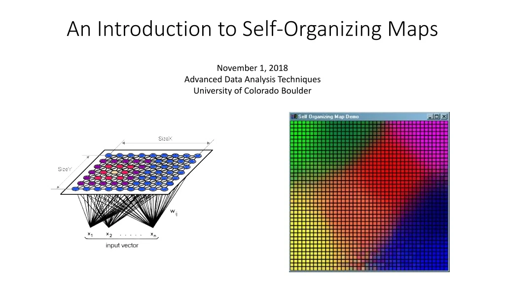
1. An Introduction to Self-Organizing Maps November 1, 2018 Advanced Data Analysis Techniques University of Colorado Boulder

2. Self-Organizing Maps - Overview • Unsupervised Neural Network • Cluster High-Dimensional Data • Contains Input Layer, Weights, Kohonen Layer • Retains the Topology of the Input Data

3. Other Clustering Methods Principal Component Analysis K Means

4. Self-Organizing Maps - Overview • Similarity between nodes • Nodes are organized in resulting map • Can capture nonlinear relationships • Nodes have physical meaning • Need to define grid size/type a priori • No method for determining best grid size • Can be computationally expensive

5. Define Terms 1 2 3 4 5 Node 1 Node 3 Node 1 Node 2 2 3 4 5 Node 25

6. Define Terms Node Weight/Code Vector

7. Define Terms Node Weight/Code Vector x,y,z Input Layer x,y,z x,y,z

8. Define Terms Node Weight/Code Vector Input Layer Kohonen Layer

9. Define Terms Node Weight/Code Vector Input Layer Kohonen Layer Best Matching Unit, BMU

10. Define Terms Node Weight/Code Vector Input Layer Kohonen Layer Best Matching Unit, BMU Neighborhood/Radius

11. Input Layer For a given observation, u, there are three variables: Sepal.Length -> x Sepal.Width -> y Petal.Length -> z

12. Learning Process

13. Learning Process Step 1: Randomly position the grid’s nodes in the data space.

14. Learning Process Data point u Step 2: Select one data point, either randomly or systematically cycling through the dataset in order

15. Learning Process Step 3: Find the node that is closest to the chosen data point. This node is called the Best Matching Unit (BMU).

16. Learning Process Step 4: Move the BMU closer to that data point. The distance moved by the BMU is determined by a learning rate, which decreases after each iteration.

17. Learning Process Step 5: Move the BMU’s neighbors closer to that data point as well, with farther away neighbors moving less. Neighbors are identified using a radius around the BMU, and the value for this radius decreases after each iteration.

18. Learning Process Step 6: Update the learning rate and BMU radius, before repeating Steps 1 to 4. Iterate these steps until positions of neurons have been stabilized.

19. SOM Learning Self-Organizing Map • Step 1: Randomly position the grid’s neurons in the data space. • Step 2: Select one data point, either randomly or systematically cycling through the dataset in order • Step 3: Find the neuron that is closest to the chosen data point. This neuron is called the Best Matching Unit (BMU). • Step 4: Move the BMU closer to that data point. The distance moved by the BMU is determined by a learning rate, which decreases after each iteration. • Step 5: Move the BMU’s neighbors closer to that data point as well, with farther away neighbors moving less. Neighbors are identified using a radius around the BMU, and the value for this radius decreases after each iteration. • Step 6: Update the learning rate and BMU radius, before repeating Steps 1 to 4. Iterate these steps until positions of neurons have been stabilized.

20. 2D Map Perspective

21. Grid Types Toroidal Grid Rectangular Grid

22. Result

23. Melt Onset Mortin et al., 2016

24. Atmospheric Rivers https://www.frontiersin.org/articles/10.3389/feart.2014.00002/full

25. Preliminary Results High # of Melt Days Low # of Melt Days count m

26. Preliminary Results – Surface Air Temperature K K

27. Preliminary Results – Surface Specific Humidity kg/kg kg/kg

28. Preliminary Results – Energy W/m^2 W/m^2

29. Preliminary Results – Day of Year

30. Thank you! Questions?