Download
1 / 40
400 likes | 579 Views
Embedded Systems: Hardware: Using Combinational Logic in Applications: Signal Levels, Time, Physical Properties; Testing, Structural and Functional Faults; Using Verilog to Model Timing Delays Main reference: Peckol, Chapter 2. Main theme of this chapter: The world is ANALOG , not digital;

E N D
Embedded Systems: Hardware: Using Combinational Logic in Applications: Signal Levels, Time, Physical Properties; Testing, Structural and Functional Faults; Using Verilog to Model Timing Delays Main reference: Peckol, Chapter 2
Main theme of this chapter: The world is ANALOG, not digital; Even in designing combination logic, we need to take analog effects into account Software doesn’t change but hardware does: --different manufacturers of the same component --different batches from the same manufacturer --environmental effects --aging --noise 3 main areas of concern: --signal levels --timing --how to deal with effects of unwanted resistance, capacitance, induction
table_02_00 SIGNAL LEVELS: “0”, “1”, and actual values “ideal”: Logical 0 = 0 volts Logical 1 = 5 volts (or 3.3 volts or …) “actual” (vendor specifications): “output >= 2.5 V to be interpreted as 1; output <= 0.4 V to be interpreted as 0 High-level noise immunity (margin) = VOH – VIH = 0.5 Low-level noise immunity (margin) = VIL –VOL = 0.4 table_02_00 0.8
fig_02_00 0 0 1 1 Logic level variations: summary (bubble = logic 0) fig_02_00 fig_02_00 fig_02_01
fig_02_02 fig_02_02 fig_02_03 fig_02_04 TTL MOS (CMOS) Typical transistor families: Q: where is the resistor in the MOS circuit? Q: why is CMOS preferred for today’s IC’s?
Fan-in: device’s input current requirements: how much current does the device source to other devices when its input is in logical 0 state; how much does it sink from other devices when input is in logical 1 state? and Fan-out: how many devices can this gate drive with out degraing its specified minimum and maximum output levels; how much current device sources to other devices in logic high state and how much it sinks from other devices in logic low state fig_02_05 Terminology: In top picture Inv1 is sourcing current to Inv2 and Inv2 is sinking current from Inv1 In bottom picture Inv2 is sourcing current to Inv1 and Inv1 is sinking current from Inv2 fig_02_05 table_02_01 Example values (SNL4LS04 data sheet)
Computing fanout for the SNL4LS04 device:: use lower of 2 values for logic 1/0 states Output = 0: can sink 8mA, source -400A; fanout =|8mA/-400A| = 20 Output 1: similar calculation gives fan-out 20 (same in this case) Example 2.0: fig_02_06 Driver driving LED and several gates; current through LED when driver is at logic 0 Specs: inverter IIL = -400A; IIH = 20uA driver: IOL = 24mA at VOL = 0.2V; IOH = -15mA at VOH = 3.5V Logic 1 (fig. 2_07): at N1, i1 + i2 + i3 = 0; LED is off i3 = i1 = 15mA; fanout = i3/i4 =15mA / 20A = 750 Logic 0 (fig 2_08): at N1, i1 + i2 + i3 = 0; LED is on i3 = i1 – i2; i3 = 15mA – 10ma = 5 mA fanout = i3/i4 = 5mA/20A = 250 fig_02_06 fig_02_08 fig_02_07
fig_02_09 Adding resistors to measure ON resistance from transistors: fig_02_09 Output: Sinking current : drop across R2 and output voltage will be above 0.0 VDC Sourcing current: drop across R1, decrease in ideal output of 5 VDC Input: Sourcing current (input = 0): drop across R3; worst case if input = 0.0 VDC; output is VOL; but making input negative can damage the part Sinking current: drop across R4. but forcing device to exceed limit can damage it.
fig_02_10 fig_02_10 TIME: rise and fall time not 0 in real life must allow for these Verilog code p. 61 //syntax # (riseTime, fallTime) deviceinstance //in part model parameter riseTime = 1; parameter fallTime = 2; Not #(riseTime, fallTime) myNot (sigOut, sigIn):
TIME: propagation delay Embedded systems : usually trying to meet a deadline, so use longest combinational delay Verilog code p. 64 //syntax // # delay LHS = RHS //RHS changes and is assigned to LHS //after a delay; //inclusion in part model (2 time units) parameter propagationDelay = 2; Not (#propagationDelay) myNot (sigIn, sigOut); //example [Q: NOT in Altera—why?] fig_02_11 fig_02_11 fig_02_12
fig_02_13 Transport and inertial delays: Transport delay model: input changes, after a specified interval, output changes Inertial delay: accounts for physical movement of electronic charge within the device: voltage level within device much reach specified minimum level before recognized as 0 or q (so signal duration must be greater than the specified minimum level); usually set to less than or equal to the propagation delay of the device fig_02_13
Race conditions and hazards (“glitches”) Critical: state or output depends on order of arrival at decision point Noncritical: output value does not depend on order of arrival of inputs Hazard: (also called a decoding spike or a glitch): present in a circuit if the circuit has the possibility of giving an incorrect output 2 types of hazards: Static: glitch may occur because of race between 2 or more input signals when output expected to remain at steady level Static-0: may produce erroneous 1; static-1: the opposite Dynamic: output may erroneously change more than once as result of one single input transition
fig_02_14 Examples: static-0 hazard: Extra delay through inverter Static-1 hazard: Adding buffers to match delays Will not work because of Parameter variations occurring In real physical parts fig_02_14
fig_02_15 Additional examples for analysis: fig_02_15
fig_02_16_01 fig_02_16_01
fig_02_16_02 fig_02_16_02
fig_02_17 Example: dynamic hazard One slow path and one fast path; other devices are assumed to have typical delays, all of the same value If B 0 1 there will be 3 state changes in the output before it settles fig_02_17
fig_02_18 fig_02_18
“LEGACY OF THE EARLY PHYSICISTS”: RESISTANCE, CAPACITANCE, COUPLING (“micro view”, passive components) Ampere: current flowing in a wire produces magnetic field Faraday, Lenz: wire moving in magnetic field has induced current Gauss et al.: capacitance Situations to examine: Coupling between two adjacent wires Mutual capacitance between adjacent circuits …etc. fig_02_19
fig_02_20 fig_02_19 PHYSICAL PROPERTIES: RESISTANCE R fig_02_19 R = r * (L / A) Q: what does this say about: --length of wires? --feature sizes? --noise margins for low voltage? Modeling resistance (first-order model, includes inherent parasitic devices): for DC, L and C can be ignored; but in our circuits we will have time-varying signals We are assuming a lumped system (all resistance considered to be “lumped” at one node) For a distributed system we would look at R(x)dx, L(x)dx, C(x)dx
fig_02_20 DC: can ignore L and C Time-changing signals: Impedance |ZL(w)| = Lw; Capacitance:|ZC(w)| = 1 / Cw Laplace transform:Z(s) = Ls + R || 1/Cs = Ls + R/(RCs + 1) Gives: for w = 0, |z(w)| = R; for w infinity, |z(w)| = L Z(w) for R = 10K, 1K, 0.1K: at ~ 10GHz, inductor becomes dominant: fig_02_21
fig_02_22 Capacitance: C = e * A/d Many instances of capacitors on chip: --Power/ground planes --parallel wires --adjacent pins --etc. Example: part of signal in top wire shows up as noise in adjacent wire: fig_02_22 fig_02_23
fig_02_24 First-order (lumped) model: Using Laplace transform gives Z(s) = 1/Cs + Ls + R; inductor dominates at higher frequencies For C = 1 muf, 0,1 muf, 0.01 muf: fig_02_24 fig_02_25
fig_02_26 How do these effects change logic circuit? Example: 2 inverters in series Resistor: connecting path Capacitor: device, wire, IC package, coupling to other devices VOUT (s) = [1/Cs] / [R + 1/Cs] * V(s)IN = [1/(RCs+1)] * V(s)IN = [1/(RCs+1)] * [VIN/s] for VIN a step function VOUT(t) = VIN(1-exp(-t/RC)) Rise (and fall) times are slowed Components can be damages or Data rate can be reduced fig_02_26 fig_02_27: interconnect fig_02_28:interconnect, driver fig_02_29: rise time
fig_02_30 Example: tristate driver Enable different data sources to use system bus If driver disables, pullup resistor controls bus VOUT(t) = VIN(1-exp(-t/RC)) Rise time is increased and Receiving device can enter metastable region where there is oscillation in its output fig_02_30 fig_02_31 fig_02_32
fig_02_33 Example: why you should never leave Gate inputs floating (using a 3-input AND gate for a 2-input application): • 1: • VOUT(s) = C1/(C1+C2)*VIN(s); • If voltage too low, output is always 0 • Cap = C1 + C2 • This doubles time constant, reduces rise/fall time; can give metastable behavior on switching • 3. State of ununsed pin defined by pullup resistor, this will work 3 methods: 1 2 3 fig_02_35 fig_02_33 fig_02_34
fig_02_36 Second-order: add parallel inductor This adds a damping factor: Natural frequency wn = 1/ (LC)1/2 ; damping d = (R/2) * (L/C)1/2 d < 1: underdamped—can have oscillation, noise; d = 1: damped okay; d > 1: overdamped—can have metastability fig_02_37 fig_02_36
fig_02_39 Testing combinational circuits Fault-unsatisfactory condition or state; can be constant, intermittent, or transient; can be static or dynamic Error: static; inherent in system; most can be caught Failure: undesired dynamic event occurring at a specific time—typically random—often occurs from breakage or age; cannot all be designed away Physical faults: one-fault model Logical faults: Structural—from interconnections Functional: within a component
fig_02_39 Structural faults: Stuck-at model: (a single fault model) s-a-1; s-a-0; may be because circuit is open or there is a short
fig_02_39 Testing combinational circuits: s-a-0 fault fig_02_39
fig_02_40 Modeling s-a-0 fault: fig_02_40
fig_02_41 S-a-1 fault fig_02_41
fig_02_42 Modeling s-a-1 fault: fig_02_42
fig_02_43 Open circuit fault; appears as a s-a-0 fault fig_02_43
fig_02_44 Bridging fault: bad connections, broken flakes, errant wire pieces fig_02_44
fig_02_45 Examples of bridging faults fig_02_45
fig_02_46 Bridging faults can be feedback or non-feedback faults Non-feedback faults Between input or output and power rail: use stuck-at model Between signal traces or logic pins: inputs: model as common signal to both inputs internal: who wins? fig_02_46
fig_02_47 Modeling a “competitive” fault: result of fault depends on logic family being used fig_02_47
fig_02_48 Feedback bridging faults: Number of inversions is important Circuit A Circuit B In A there are an odd number of inversions on the path; this can cause oscillation; can sometimes be modeled as competing signals In B there are an even number of inversions; this can oftn be modeled as a stuck-at fault fig_02_48
fig_02_49 Functional faults: Example: hazards, race conditions Two possible methods: A: consider devices to be delay-free, add spike generator B: add delay elements on paths Method A Method B As frequencies increase, eliminating hazards through good design iseven more important fig_02_49 fig_02_50