Embedded Systems: Hardware Combinational Logic (Peckol 2.5-2.8 & 10.11-10.15 + notes) Testing

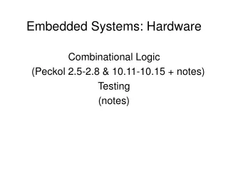
1. Embedded Systems: Hardware Combinational Logic (Peckol 2.5-2.8 & 10.11-10.15 + notes) Testing (notes)

2. Main issues in performance of combinational logic: The world is ANALOG, not digital; even in designing combination logic, we need to take analog effects into account Software doesn’t change but hardware does: --different manufacturers of the same component --different batches from the same manufacturer --environmental effects --aging --noise main areas of concern: --signal levels (“0”, “1”—min, typical, and max values; fan-in, fan-out) --timing—rise & fall times; propagation delay; hazards and race conditions --how to deal with effects of unwanted resistance, capacitance, induction

3. Race conditions and hazards (“glitches”) Critical: state or output depends on order of arrival at decision point Noncritical: output value does not depend on order of arrival of inputs Hazard: (also called a decoding spike or a glitch): present in a circuit if the circuit has the possibility of giving an incorrect output 2 types of hazards: Static: glitch may occur because of race between 2 or more input signals when output expected to remain at steady level Static-0: may produce erroneous 1; static-1: the opposite Dynamic: output may erroneously change more than once as result of one single input transition

4. fig_02_14 Examples: static-0 hazard: Extra delay through inverter Static-1 hazard: Adding buffers to match delays Will not work because of Parameter variations occurring In real physical parts fig_02_14

5. fig_02_15 Additional examples for analysis: fig_02_15

6. fig_02_16_01 fig_02_16_01

7. fig_02_16_02 fig_02_16_02

8. fig_02_17 Example: dynamic hazard One slow path and one fast path; other devices are assumed to have typical delays, all of the same value If B 0  1 there will be 3 state changes in the output before it settles fig_02_17

9. fig_02_18 fig_02_18

10. “LEGACY OF THE EARLY PHYSICISTS”: RESISTANCE, CAPACITANCE, COUPLING (“micro view”, passive components) Ampere: current flowing in a wire produces magnetic field Faraday, Lenz: wire moving in magnetic field has induced current Gauss et al.: capacitance Situations to examine: Coupling between two adjacent wires Mutual capacitance between adjacent circuits …etc. fig_02_19

11. fig_02_20 fig_02_19 PHYSICAL PROPERTIES: RESISTANCE R fig_02_19 R = r * (L / A) Q: what does this say about: --length of wires? --feature sizes? --noise margins for low voltage? Modeling resistance (first-order model, includes inherent parasitic devices): for DC, L and C can be ignored; but in our circuits we will have time-varying signals We are assuming a lumped system (all resistance considered to be “lumped” at one node) For a distributed system we would look at R(x)dx, L(x)dx, C(x)dx

12. fig_02_22 Capacitance: C = e * A/d Many instances of capacitors on chip: --Power/ground planes --parallel wires --adjacent pins --etc. Example: part of signal in top wire shows up as noise in adjacent wire: fig_02_22 fig_02_23

13. fig_02_24 First-order (lumped) model: Using Laplace transform gives Z(s) = 1/Cs + Ls + R; inductor dominates at higher frequencies For C = 1 muf, 0,1 muf, 0.01 muf: fig_02_24 fig_02_25

14. fig_02_26 How do these effects change logic circuit? Example: 2 inverters in series Resistor: connecting path Capacitor: device, wire, IC package, coupling to other devices VOUT (s) = [1/Cs] / [R + 1/Cs] * V(s)IN = [1/(RCs+1)] * V(s)IN = [1/(RCs+1)] * [VIN/s] for VIN a step function VOUT(t) = VIN(1-exp(-t/RC)) Rise (and fall) times are slowed Components can be damaged or Data rate can be reduced fig_02_26 fig_02_27: interconnect fig_02_28:interconnect, driver fig_02_29: rise time

15. fig_02_30 Example: tristate driver Enable different data sources to use system bus If driver disables, pullup resistor controls bus VOUT(t) = VIN(1-exp(-t/RC)) Rise time is increased and Receiving device can enter metastable region where there is oscillation in its output fig_02_30 fig_02_31 fig_02_32

16. fig_02_33 Example: why you should never leave Gate inputs floating (using a 3-input AND gate for a 2-input application): • 1: • VOUT(s) = C1/(C1+C2)*VIN(s); • If voltage too low, output is always 0 • Cap = C1 + C2 • This doubles time constant, reduces rise/fall time; can give metastable behavior on switching • 3. State of unused pin defined by pullup resistor, this will work 3 methods: 1 2 3 fig_02_35 fig_02_33 fig_02_34

17. fig_02_36 Second-order: add parallel inductor This adds a damping factor: Natural frequency wn = 1/ (LC)1/2 ; damping d = (R/2) * (L/C)1/2 d < 1: underdamped—can have oscillation, noise; d = 1: damped okay; d > 1: overdamped—can have metastability fig_02_37 fig_02_36

18. fig_02_39 Testing combinational circuits Fault-unsatisfactory condition or state; can be constant, intermittent, or transient; can be static or dynamic Error: static; inherent in system; most can be caught Failure: undesired dynamic event occurring at a specific time—typically random—often occurs from breakage or age; cannot all be designed away Physical faults: one-fault model Logical faults: Structural—from interconnections Functional: within a component

19. fig_02_39 Structural faults: Stuck-at model: (a single fault model) s-a-1; s-a-0; may be because circuit is open or there is a short

20. fig_02_39 Testing combinational circuits: s-a-0 fault fig_02_39

21. fig_02_40 Modeling s-a-0 fault: fig_02_40

22. fig_02_41 S-a-1 fault fig_02_41

23. fig_02_42 Modeling s-a-1 fault: fig_02_42

24. fig_02_43 Open circuit fault; appears as a s-a-0 fault fig_02_43

25. fig_02_44 Bridging fault: bad connections, broken flakes, errant wire pieces fig_02_44

26. fig_02_45 Examples of bridging faults fig_02_45

27. fig_02_46 Bridging faults can be feedback or non-feedback faults Non-feedback faults Between input or output and power rail: use stuck-at model Between signal traces or logic pins: inputs: model as common signal to both inputs internal: who wins? fig_02_46

28. fig_02_47 Modeling a “competitive” fault: result of fault depends on logic family being used fig_02_47

29. fig_02_48 Feedback bridging faults: Number of inversions is important Circuit A Circuit B In A there are an odd number of inversions on the path; this can cause oscillation; can sometimes be modeled as competing signals In B there are an even number of inversions; this can often be modeled as a stuck-at fault fig_02_48

30. fig_02_49 Functional faults: Example: hazards, race conditions Two possible methods: A: consider devices to be delay-free, add spike generator B: add delay elements on paths Method A Method B As frequencies increase, eliminating hazards through good design iseven more important fig_02_49 fig_02_50

31. Testing: • General Requirements • DFT • Multilevel Testing-- • System, Black Box, White Box Tests

32. Testing--General Requirements • Testing--general requirements: • thorough • ongoing • DEVELOPED WITH DESIGN (DFT--design for test) • note: this implies that several LEVELS of testing will be carried out • efficient

33. Good, Bad, and Successful Tests • good test: has a high probability of finding an error • ("bad test": not likely to find anything new) • successful test: finds a new error

34. Most Effective Testing Is Independent most effective testing: by an "independent” third party Question: what does this imply about your team testing strategy for the quarter project?

35. How Thoroughly Can We Test? how thoroughly can we test? example: VLSI chip 200 inputs 2000 flipflops (one-bit memory cells) # exhaustive tests? What is the overall time to test if we can do 1 test / msec? 1 test / msec? 1 test /nsec?

36. Design for Testability (DFT)--what makes component "testable"? • operability: few bugs, incremental test • observability: you can see the results of the test • controllability: you can control state + input to test • decomposability: you can decompose into smaller problems and test each separately • simplicity: you choose the “simplest solution that will work” • stability: same test will give same results each time • understandability: you understand component, inputs, and outputs Design for Testability (DFT)

37. Testing strategies testing strategies: verification--functions correctly implemented validation--we are implementing the correct functions (according to requirements)

38. A general design/testing strategy can be described as a "spiral”: requirements  design  code system test module,integ. tests unit test (system) (black (white box) box) when is testing complete? One model: "logarithmic Poisson model” f(t)=(1/p)ln(I0pt+1) f(t) = cumulative expected failures at time t I0 = failures per time unit at beginning of testing p = reduction rate in failure intensity Spiral design/testing strategy Design/Module Tests Implement/Unit Tests Design/Integration Tests START END Requirements, Specs/System Tests

39. Types of testing: • white box--"internals” (also called "glass box") • black box—modules and their "interfaces” (also called "behavioral") • system--”functionality” (can be based on specs, use cases) • (application-specific) Types of testing

40. steps in good test strategy: • quantified requirements • test objectives explicit • user requirements clear • use "rapid cycle testing" • build self-testing software • filter errors by technical reviews • review test cases and strategy formally also • continually improve testing process Good testing strategy

41. Black box testing guidelines General guidelines: test BOUNDARIES test output also choose "orthogonal” cases if possible