Simulation and Feedback Control in Atomic Force Microscope Presentation
Explore AFM components, feedback control techniques, interaction forces, noise sources, and detection methods in AFM simulations. Understand the complexities in position control and noise reduction strategies to enhance AFM performance.

Simulation and Feedback Control in Atomic Force Microscope Presentation
E N D
Presentation Transcript
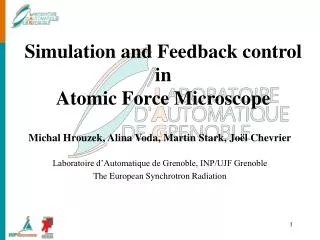
Simulation and Feedback control in Atomic Force Microscope Michal Hrouzek, Alina Voda, Martin Stark, Joël Chevrier Laboratoire d’Automatique de Grenoble, INP/UJF Grenoble The European Synchrotron Radiation
Outlines of the presentation • AFM description • Feedback control in AFM • Sources of noise in AFM • Cantilever model • Driving loop with controller • Interaction forces • Thermal noise in AFM • Conclusion
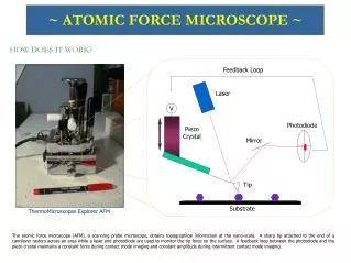
Schema of Dynamic Force Microscopy (excitation) • Head of the AFM • Driving loop • Head positioning loop • Stage with a sample • x axis positioning loop • y axis positioning loop (set-value of Dw)
Detection techniques in dynamic AFM • Amplitude Modulation (AM) • Original operation technique, Developed by Y. Matin – J. Appl. Phys. 61 (10) • Driver is exciting the cantilever with constant driving signal. • Interaction forces affect the cantilever and lower the vibration amplitude. • Change in amplitude depends directly on interaction force. • Frequency Modulation (FM) • Newer technique, Developed by T.R. Albrecht – J. Appl. Phys. 69 (2) • Driver with controller is exciting the cantilever to constant vibration amplitude. • Interaction forces affect the cantilever and change the resonant frequency. • Frequency shift depends directly on interaction force. Dw Df • More sensitive compare to AM-technique • Further would be treated only FM technique.
Outlines of the presentation • AFM description • Feedback control in AFM • Sources of noise in AFM • Cantilever model • Driving loop with controller • Interaction forces • Thermal noise in AFM • Conclusion
Feedback control in AFM • Loop controlling position of AFM head in z axis • Maintaining constant set-value of frequency shift • Low frequency response (1 – 30 kHz) • Cantilever driving loop (cantilever excitation) • Exciting the cantilever and ensuring that contact with surface is not lost • High frequency response (1kHz – 1 MHz) • Nonlinear behavior of the driver (due coupling with surface) • Directly maintaining cantilever vibration amplitude • Could be used for possible attenuation of thermal noise perturbation and influence of another noises.
Position of the head and lever excitation rzd(t), rzp(t) – desired excitation and set-value of frequency shift mz(t) – measured deflection of the cantilever ezd(t), ezp(t) – regulation errors of the bimorph and head zdri(t), zpos(t) – driving signal and head positioning signal z(t) – real deflection of the cantilever
Feedback control in AFM • Loops controlling position of AFM stage in x-y axes • Scanning • Positioning of the stage with sample • Simple movement in straight lines under the cantilever with tip • Manipulation • Particles manipulation at the surface • Complex movement with many possible shapes • Control of the applied force onto the particle is crucial Scanning Manipulation
Loops controlling stage position rx,y(t) – desired position piezo-electric stack mx,y(t) – measured (estimated) position of the stage ex,y(t) – regulation error ux,y(t) – driving signal yx,y(t) – real position of the stage
Loops controlling stage position • Accuracy problems with piezo-electric actuators • Positioning nonlinearities (getting bigger with increasing speed) • Usually are used piezo stacks with hysteresis 10% - 15% of max. displacement (Harder stacks have smaller hysteresis but smaller displacement range) • Drift due to creep (Could be reduced to curtain level by careful design of the stage) • Measurement problems of stage position • High level of noise of LVDT detectors get relevant at nano-meter resolution • Observer based regulator can achieve better positioning resolution
Outlines of the presentation • AFM description • Feedback control in AFM • Sources of noise in AFM • Cantilever model • Driving loop with controller • Interaction forces • Thermal noise in AFM • Conclusion
Sources of noise in AFM • Electronic parts • Photo detector • Optical path noise • Thermal gradient • Laser intensity noise • Shot noise • Laser mode noise • Laser phase noise • Electronic circuits • Electrostatic noises • Noise of amplifiers • Mechanical parts • Cantilever and tip • Thermally induced cantilever noise • Mechanical vibration • Relaxation • Air turbulences and acoustic waves • Magnetic noises • Electrostatic noises • Chemical noises • Bimorph • Thermally induced noise • Electrostatic noises
Thermal noise • Thermal noise is limiting AFM sensitivity Some noises could be lower by appropriate design and construction of AFM. • The minimum detectable interaction force.(dynamic mode) • k Spring constant, stiffness • T Temperature • kB Boltzmann constant • b Measurement bandwidth • A0 Vibration amplitude • w0 Resonance frequency • Q Quality factor
Outlines of the presentation • AFM description • Feedback control in AFM • Sources of noise in AFM • Cantilever model • Driving loop with controller • Interaction forces • Thermal noise in AFM • Conclusion
Cantilever model • Second order differential equation model • Q 0.1-1 liquid environment 1-1000 air environment 1000-100000 vacuum environment • L 10-500mm length • w 10-50mm width • t 0.1-5mm thick • E 130-180GPa for silicon cantilevers • k 0.01-100N/m stiffness
Cantilever model • Multimode model of the cantilever • E Modulus of elasticity • I Area moment of inertia • m Mass per unit length • L Cantilever length
Cantilever model • Multimode model of the cantilever • E Modulus of elasticity • I Area moment of inertia • m Mass per unit length • L Cantilever length
Computer Simulation • The cantilever properties used for multimode model • Computed properties of separated harmonic modes
Computer Simulation • Spectral analysis schema of the multi mode cantilever model
Computer Simulation - results • Thermal noise was the only excitation of the Cantilever. (displayed spectra is an average over 100 FFT)
Measured spectra • non-contact silicon cantilever NSC12/50 (cantilever F) (displayed spectra is an average over 1000 FFT)
Computer Simulation - results • Time response of thermally driven cantilever -Time sequence 0 to 2ms -Time sequence 0 to 0.2ms (Zoom) Zoom Model initialization Modeled thermal excitation (blue) (normal distribution) Position of the cantilever (red)
Computer Simulation - results • Time response of artificially driven cantilever at resonance blue curve – exciting displacement zdriv(t)=Z0sin(w0t) red curve – displacement of the cantilever at its free end - Time sequence 0 to 10ms - Time sequence 0 to 0.4ms (zoom) Zoom
Outlines of the presentation • AFM description • Feedback control in AFM • Sources of noise in AFM • Cantilever model • Driving loop with controller • Interaction forces • Thermal noise in AFM • Conclusion
Computer Simulation with controller Driving with the PID regulator
Computer Simulation with controller • Driver with phase shift • Band pass filter – selects the frequencies of our interest (10kHz-100kHz) • Amplitude detector – gives numerical value of vibration amplitude A(t) • Controller – select the gain(t) that is multiplied by filtered cantilever position • Low pass filter – eliminates high frequency noise • Gain – amplification of the signal • Phase shift – optimal value is p/2
Computer Simulation with controller - results Gain of the PID controllergain(t)
Computer Simulation with controller - results Displacement of the driving bimorph zbimorph(t) = kbimorph zdrive(t)
Computer Simulation with controller - results Displacement of the cantilever (red curve) Displacement of the driving bimorph (blue curve)
Outlines of the presentation • AFM description • Feedback control in AFM • Sources of noise in AFM • Cantilever model • Driving loop with controller • Interaction forces • Thermal noise in AFM • Conclusion
Interaction forces • Properties • They are non-linear • Can be long-range or short-range, and attractive or repulsive. • Forces are very sensitive to environmental conditions such as temperature, humidity, surface chemistry, and mechanical and electrical noises. • Depend on the material, geometry and size of nano entities. • Curtain forces are getting dominant in specific environments and some diminish. • Interaction forces • van der Waals (analogous to the gravity at the nano-scale) • Casimir • Thermal motion: Exist for any material and depends only on temperature • Capillary, Hydrogen and Covalent bonding, Steric, Hydropobolic, Double layer, …
Interaction forces • Intensity of the van der Waals and repulsive forces.
Interaction forces • Approach curve of the cantilever. 1) Non-contact 2) “Snap on” point, spring constant is smaller than attractive force. zero) Equilibrium point, lever isn’t deflected in any direction. 3) Repulsive interaction is dominant. 4) Maximum positive deflection. 5) Capillarity holds the tip onto the surface 6) “snap off” point, spring constant overcomes the capillarity
Interaction forces model • Mathematical equations describing interaction forces between the tip and surface • Intensity of the interaction forces as a function of the separation distance. a0– intermolecular distance AH – Hamaker constant RS – Sphere radius (end of the tip) E* – Effective stiffness • Numerical values used from reference: S. I. Lee, Physical Review B, 66(115409), 2002.
Interaction forces model - results • Approach curve is simulated without any excitation, chip with the cantilever is slowly approaching the surface Approach curve with the cantilever, Q=1 Approach curve with the cantilever, Q=100 • This behavior has been observed at the experiment. (Martin Stark, Frederico Martins)
Interaction forces model - results Cantilever has been excited with constant driving signal zbimorph(t) = Adrivesin(w0t) Harmonic outputs of separated modes has been recorded. Amplitude of first harmonic mode is decreasing with smaller separation distance. Vibration amplitude Separation distance
Interaction forces model - results • Amplitude of higher harmonic modes are increasing with smaller separation distance. • Time sequences of one period are shown (second mode – red curve, third mode – green curve, fourth mode – blue curve )
Outlines of the presentation • AFM description • Feedback control in AFM • Sources of noise in AFM • Cantilever model • Driving loop with controller • Interaction forces • Thermal noise in AFM • Conclusion
Outlines of the presentation • AFM description • Feedback control in AFM • Sources of noise in AFM • Cantilever model • Driving loop with controller (model of PLL) • Interaction forces • Thermal noise in AFM • Conclusion
Conclusion • Multimode cantilever model has been developed. Simulations have shown that the model is correct approximation of the dynamic system. • Model of the interaction forces have been implemented into Matlab Simulink environment. • Dynamic interaction between both models has been simulated and compared with measurements. • Driving controller has been employed to control the excitation of the cantilever interacting with the surface.
Acknowledgements • Frederico Martins • Mario Rodrigues • Raphaelle Dianoux
Future work • Development of microscope stage controllers that are responsible for the sample positioning under the head with cantilever. This controller has to fulfill new requirements for speed and accuracy due to application of the AFM as a nano-manipulator. • Thermal noise is second field of further work. Driving controller has to be redesigned to lower the nose signal ration to achieve better results in weak forces measurements.