SPATIAL PATTERN
SPATIAL PATTERN. Compiled by Dr. Esra Ozdenerol Advanced GIS 4525-6525.

SPATIAL PATTERN
E N D
Presentation Transcript
SPATIAL PATTERN Compiled by Dr. Esra Ozdenerol Advanced GIS 4525-6525
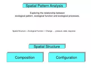
Geographers often examine spatial patterns on the earth’s surface produced by physical or cultural processes. These patterns represent the spatial distribution of a variable across a study area. Sometime geographic variables are displayed as point patterns. Whether data are presented as points or areas, geographers often want to describe and explain an existing pattern.
Point Pattern Analysis in GIS • A common body of knowledge of point pattern analysis exists in the geographical, forestry and other sciences. Nevertheless, structural point pattern analysis is quite limited in geographic information systems. Present commercial GIS use elaborate techniques for spatial operations like buffering objects or overlaying different thematic layers.
Concerning statistical spatial analysis of point objects, their capabilities are limited to simple descriptive measures such as minimum, maximum, mean and standard deviation. • Some raster-based systems (e.g., IDRISI) offer more complex statistical analysis functions (e.g. measures of spatial autocorrelation), but they do not offer sophisticated algorithms for point pattern analysis.
Several authors (Goodchild et al., 1991; Openshaw 1991)discuss possible ways to link GIS with statistical spatial analysis. Five strategies may be distinguished: • free standing spatial analysis systems • integration of basic GIS functionality to statistical software • 'loose coupling' of proprietary GIS to statistical software • 'close coupling' of GIS and statistical software • complete integration of statistical spatial analysis in GIS
The second strategy is applied in the experimental system SPLANCS by Rowlingson and Diggle (1993). They made some enhancements to the S-Plus system to produce a tool for display and analysis of spatial point pattern data. G-, F- and K-functions as well as a kernel smoothing procedure were implemented. The advantage of having the full statistical capabilities of S-Plus available is achieved at the expense of having no real GIS functionality. This approach, although criticized by Openshaw (1991), has also been adopted by Griffith (in Haining and Wise, 1991) and SAS Inc. producing a module SAS/GIS.
Several developments try to couple GIS with commercially available statistical packages such as GLIM, SAS, SPSS, generally using ASCII exports. They mostly concentrate on measures of spatial autocorrelation and association (Gatrell and Rowlingson 1994). Others implemented methods for point pattern analysis concentrating on first- and second-order analysis (MacLennan 1991; ; Rowlingson and Diggle 1993; Gatrell and Rowlingson 1994); they occasionally include some density estimation techniques (e.g., kernel density estimation).
MacLennan 1991 implemented second-order analysis methods (G- and L-functions) into the GRASS system (GRASS 1993). Analysis of time aspects has rarely been considered, partly because of the lack of infrastructure for temporal geographic information systems and the absence of established analysis methods.
Openshaw 1994 presents a new analysis approach by extending his earlier work to 'geographical analysis machines' GAM (Openshaw 1987). He argues that traditional exploratory methods of pattern discovery are not feasible in a multivariate GIS environment with tri-space (geographical, temporal and attribute) information. He extends his GAM to 'space-time-attribute-machines' (STAM) and '-creatures' (STAC), using artificial life (see Langton 1989; Beer 1990) to search all three spaces (Openshaw and Perree 1996). Basically, a STAM is an automatic screening program which is searching all the locations in geography, time and attribute space for evidence of clustering.
Geographers may want to compare an existing spatial pattern to a particular theoretical pattern. Spatial patterns may appear clustered, dispersed, or random.
In case 1, both the point and area patterns have a clustered appearance. Perhaps the points represent sites of Economic activity(retail and service functions), which often cluster around a Location with high accessibility and high profit potential, such as highway interchange. On the clustered area pattern map, the shaded sub areas could represent political precincts where a majority of registered voters are democrat. Such as clustered pattern would likely occur if there is a distinctly nonrandom spatial distribution of voters by income, race, or ethnicity in the region.
The set of points in case 2 appears uniformly distributed across the study area, Suggesting that a systematic spatial process produced the locational pattern. The pattern exhibits a regular or alternating type of spatial arrangement. The hypothesis In classical central place theory, for example, is that settlements are uniformly distributed across the landscape to best serve the needs of a dispersed rural population. This pattern could represent county populations in the same region where the central place distribution of settlements is hypothesized.Shaded counties could have above average populations while unshaded counties are below average.
The spatial patterns in case 3 appear random in nature, with no dominant trend toward either clustering or dispersion. A random point or area pattern logically suggests that a spatially random (Poisson) process is operating to produce the pattern.
Nearest Neighborhood Analysis = = = The distance of each point to its nearest neighbor is measured and the average nearest neighbor distance for all points is determined.For each of the points, NN is determined as the point closest in Straight line(Euclidean) distance. PointxyNNNND A 1.3 0.9 B 3.98 B 3.2 4.4 C 2.00 C 3.3 6.4 B 2.00 D 5.6 3.8 E 1.36 E 4.8 2.7 D 1.36 F 8.1 7.4 G 4.21 G 9.4 3.4 F 4.21 Sum19.12 === = = = = NN= Nearest Neighbor NND= Nearest Neighbor Distance Average Nearest Neighbor Distance
= = = 1.89 = = 1.44 If points are arranged in a random spatial pattern, the average nearest neighbor distance would be determined as follows: = Density=number of points (n)/Area The area represented is 100 square units. Density of points is therefore 7/100=.07. R==1.44 ==1.89 R==1.44 R This spacing pattern is moderately dispersed, since it lies between a perfectly dispersed distribution and a random one. Although the minimum value of the nearest neighbor index is always 0(a perfectly clustered pattern), the maximum value Corresponding to a perfectly dispersed pattern is not constant, But a function of the point density. To overcome this, a Standardized nearest neighbor index (R) is often used.
Quadrat Analysis = = S2 = VMR = A set of quadrats or square cells is superimposed on the study area, and the number of points in each cell is determined. Whereas NNA concerns the average spacing of the closest points, QA considers the variability in the number of points per cell. In QA, an index known as the variance-mean ratio (VMR) standardizes the degree of variability in cell frequencies relative to the mean cell frequency: Where: VMR=variance-mean ratio VAR= variance of the cell frequencies MEAN= mean cell frequency
If each of the quadrats contains the same number of points (case 1), the pattern would show no variability in frequencies from cell to cell and would be perfectly dispersed. By contrast, if a wide disparity exists in the number of points per cell for the set of quadrats examined (case 2), the variability of cell frequencies would be large, and the pattern would display a clustered arrangement. In case 3, the variability of cell frequencies is moderate,the pattern of points reflect random or near random spatial arrangement.
X2=VMR(m-1) In addition to its use as a descriptive index, the variance-mean ratio can also be applied inferentially to test a distribution for randomness. The test Statistic is chi-square, defined as a function of both the VMR and number of cells(m).
Different cell sizes produce varying levels of the mean point frequency and variance per cell.
AREA PATTERN ANALYSIS: Spatial Autocorrelation Spatial autocorrelation measures the degree to which a spatial phenomenon correlates to itself in space, and is considered a fundamental descriptor of the spatial structure of the phenomenon. Measuring the spatial autocorrelation helps determine how the high and low values are arranged in space. In general, if high values of a variable in one area areassociated with high values of that variable in neighboring areas, the spatialpattern exhibits positive spatial autocorrelation for that variable. Conversely, when high and low values alternate at neighboring areas, the spatial autocorrelation is negative (Goodchild 1986). The Moran’s I and Geary’s C indexes are the two spatial autocorrelation measures. == S2 =
32 white cells, 32 black cells, but spatial distribution is different a illustrates extreme negative autocorrelation between cells. e shows positive autocorrelation, cells cluster together into a homogeneous regions. c spatial independence, an autocorrelation of 0 b relatively dispersed arrangement d relatively clustered one.
Scale matters….. The degree of spatial autocorrelation present in a pattern is very much dependent on scale. If were were to subdivide each cell into four and measure the autocorrelation between neighboring cells the results would be quite different, although the pattern is the same. So any measurement of Spatial autocorrelation must be specific to a particular scale, and a pattern can have different amounts at different scales.
8/4 = 2 = = Example dataset for calculation of the Geary and Moran coefficients Example calculation of the Geary Index: w= 0 1 1 1 1 0 0 1 1 0 0 1 1 1 1 0 n=4 Z1=3 Z2=2 z3=2 Z4=1 = ==8/4=2 c= 0 1 1 4 1 0 0 1 1 0 0 1 4 1 1 0 Cij=(zi-zj)2 =0x0+1x1+1x1+1x4+1x1+0x0+0x0+1x1+ 1x1+0x0+0x0+1x1+1x4+1x1+1x1+0x0 =16
=10 = 2 / 3 = / =16 /2x(2/3)x10 =1.200 2 C= c > 1 Dissimilar Moran’s Index(Moran 1948) provides an alternative to Geary’s C for the same data context, in most applications both are equally satisfactory. Perhaps the only obvious advantage of one over the other is that Moran index is arranged so that its extremes match the intuitive notions of positive and negative correlation, whereas Geary’s index uses a more confusing scale. Moran’s index is positive when nearby areas tend to be similar in attributes, negative when they tend to be more dissimilar than one might expect, and approximately zero when attribute values are arranged randomly and independently in space. = = ==8/4=2 =
Corresponce between Geary, Moran and conceptual scales of spatial autocorrelation Geary c Moran I Similar, regionalized Smooth, clustered 0 < c < 1 I > 0* Independent, uncorrelated c = 1 I = 0 Random Dissimilar, contrasting, Checkerboard c > 1 I < 0* * The precise expectation is –1/(n-1) rather than 0.
Cij=( Zi- ) (ZJ- The attribute similarity measure used by the Moran index makes it analogous to a Covariance between the values of a pair of objects: c= 1 0 0 -1 0 0 0 0 0 0 0 0 -1 0 0 1 ) I = / = 2/ 4 = 0.5 = -2 = I = / = -2 / 0.5 x 10 = - 0.400 I < 0* Dissimilar
References Gatrell, A. and Rowlingson, B. (1994). Spatial point process modelling in a GIS environment. Taylor and Francis, London. Goodchild, M., Haining, R., and Wise, S. (1991). Integrating gis and spatial data analysis: problems and possibilities. International Journal of Geographical Information Systems, 6:407-23. GRASS (1993). GRASS 4.1 User's Reference Manual. USACERL. Haining, R. and Wise, S. (1991). Gis and spatial data analysis. Report on the Sheffield Workshop. Discussion Paper 11. University o Intelligence as Adaptive Behaviour: An experiment in Computational Neuroenthology. Langton, C. (1989). Artificial Life. Addison-Wesley. MacLennan, M. J. (1991). The use of a geographic information system for second-order analysis of spatial point patterns. Sheffield Academic Press. . Rowlingson, B. and Diggle, P. (1993). Splancs: Spatial point pattern analysis code in s-plus. Computers and Geosciences, 19(5):627-655.
References cont… • Openshaw, S. (1987). A mark 1 geographical analysis machine for the automated analysis of point data sets. International Journal of GIS, 1:335-358. • Openshaw, S. (1994). Spatial Analysis and GIS., chapter Exploratory space-time-attribute pattern analysers. Taylor and Francis., London. • Openshaw, S. and Perrée, T. (1996). Innovations ins GIS 3, chapter User-centred intelligent spatial analysis of point data., pages 119-134. Taylor and Francis, London. • Beer, R. (1990).