Download
1 / 72
720 likes | 751 Views
Chapter 2. Waiting Lines and Queuing Theory Models. Learning Objectives. Students will be able to: Describe the trade-off curves for cost-of-waiting time and cost-of-service. Explain the three parts of a queuing system: the calling population, the queue itself, and the service facility.

E N D
Chapter 2 Waiting Lines and Queuing Theory Models
Learning Objectives Students will be able to: • Describe the trade-off curves for cost-of-waiting time and cost-of-service. • Explain the three parts of a queuing system: the calling population, the queue itself, and the service facility. • Explain the basic queuing system configurations. • Describe the assumptions of the common queuing system models. • Analyze a variety of operating characteristics of waiting lines.
Chapter Outline 5.1 Introduction. 5.2 Waiting Line Costs. 5.3 Characteristics of a Queuing System. 5.4 Single-Channel Queuing Model with Poisson Arrivals and Exponential Service Times (M/M/1). 5.5 Multi-Channel Queuing Model with Poisson Arrivals and Exponential service Times (M/M/m). 5.6 Constant Service Time Model (M/D/1). 5.7 Finite Population Model (M/M/1 with Finite Source). 5.8 Some General Operating Characteristics Relationships. 5.9 More Complex Queuing Models and the Use of Simulation.
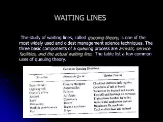
1. Introduction Queuing theoryis one of the most widely used quantitative analysis techniques. The three basic components are: • Arrivals, • Service facilities, • Actual waiting line. Waiting line problems are centered on the questions of finding the ideal level of services that the firm should provide.
1. Introduction (Cont’d.) - Supermarkets, decides how many cash register check out positions opened. - Gasoline stations, the number of pumps opened. - Manufacturing plants, the optimal number of mechanics to have on duty for repair. - Banks, the number of teller windows to keep open to serve customers in various hours of a day.
2. Waiting Line Costs Queuing analysis includes: • Determining the best level of service. • Analyzing the trade-off between cost of providing service and cost of waiting time. • Most managers want queues that are short enough so that customers do not become unhappy. • One means of evaluating a service facility is to look at a total expected cost, which is the sum of expected service cost plus expected waiting cost, see the following figure:
Queuing Costs and Service Levels Optimal Service Level Total Expected Cost Cost Cost of Providing Service Cost of Waiting Time Service Level
Three Rivers Shipping Co. Example The superintendent at Three Rivers Shipping Company wants to determine the optimal number of stevedores to employ each shift. Number of Stevedores Working 1 2 3 4 (a) Avg. number of ships arriving per shift 5 (b) Average waiting time per ship to be unloaded (hours) 7 4 3 2 (c) Total ship hours lost per shift (a × b) 35 20 15 10 (d) Estimated cost per hour of idle ship time $1,000 (e) Value of ship’s lost time (c × d) $15,000 $10,000 $35,000 $20,000 $6,000 $12,000 $18,000 $24,000 (f) Stevedore teams salary $32,000 $41,000 $33,000 $34,000 (g) Total expected cost (e+f)
3. Characteristics of a Queuing System • Arrival Characteristics: • Size of the calling population. • Pattern of arrivals. • Behavior of arrivals. • Waiting Line Characteristics: • Queue length. • Queue discipline. • Service Facility Characteristics: • Configuration of the queuing system. • Service time distribution.
Arrival Characteristics of a Queuing System • Calling Population: • Unlimited (infinite). • Limited (finite). • Arrival Pattern: • Randomly. • Poisson Distribution.
.35 .30 .25 .20 .15 .10 .05 .00 Arrival Characteristics:Poisson Distribution For X = 0, 1, 2, 3, 4, … P(X), = 2 P(X), = 4 P(X) .30 P(X) .25 .20 .15 .10 .05 .00 0 1 2 3 4 5 6 7 8 9 10 11 0 1 2 3 4 5 6 7 8 9 10 X X
Arrival Characteristics of a Queuing System (continued) Behavior of arrivals: • Join the queue, wait till served, and do not switch between lines. • Balk; refuse to join the line. • Renege (Withdraw); enter the queue, but then leave without completing the transaction.
Waiting Line Characteristics of a Queuing System Waiting Line Characteristics: • Length of the queue: • Limited. • Unlimited. • Service priority/Queue discipline: • First In First Out (FIFO). • Other.
Service Facility Characteristics • Configuration of the queuing system: • Number of channels (servers): • Single. • Multiple. • Number of phases in service system (customer stations): • Single (1 stop). • Multiple (2+ stops). • Service time distribution: • Exponential. • Other.
Service Characteristics: Queuing System Configurations Queue Service facility arrivals Departure after Service A bank which has only one open teller. Single Channel, Single Phase Service Facility Queue arrivals Facility 2 Facility 1 Departure after Service Single Channel, Multi-Phase
Service Characteristics: Queuing System Configurations Service facility 1 Queue Service facility 2 Service facility 3 Multi-Channel, Single Phase System arrivals Departure after Service Type 2 Service Facility Type 1 Service Facility Queue arrivals Type 1 Service Facility Type 2 Service Facility Multi-Channel, Multiphase System Departure after Service
Service Characteristics of a Queuing System Service Time Patterns: • Exponential probability distribution. • Other distributions.
Service Time Characteristics:Exponential Distribution Probability Average Service Time of 20 Minutes Average Service Time of 1 Hour 30 60 90 120 150 180 Service Time (Minutes), X
Identifying Models Using Kendall Notation The basic three-symbol Kendall notation: Where: M = Poisson distribution for the number of occurrences (or exponential times). D = Constant (deterministic rate). G = General distribution with mean and variance known. Arrival Service Time Number of Service Distribution Distribution Channels Open A Single channel model with Poisson arrivals and exponential service times. M/M/1 M/M/2 When a second channel is added
Identifying Models Using Kendall Notation (Cont’d.) • If there are mdistinct service channels in the queuing system with Poisson arrivals and exponential service times, the Kendall notations will be: • A three channel system with poisson arrivals and constant service time is: • A four-channel system with Poisson arrivals and service times that are normally distributed would be: M / M/ m M / D/ 3 M / G/ 4
4. Single-Channel Queuing Model with Poisson Arrivals and Exponential Service Times (M / M/ 1) Assumptions of the Model: 1. Queue discipline: FIFO. 2. No balking or reneging. 3. Arrivals: Poisson distributed. 4. Independent arrivals; constant rate over time. 5. Service times: exponential, average known. 6. Average service rate > average arrival rate.
Operating Characteristics of Queuing Systems • Average number of customers in the system (L). • Average time each customer spends in the system (W). • Average length of the queue (Lq). • Average time each customer spends waiting in the queue (Wq). • Utilization factor for the system (ρ). • Probability that the service facility will be idle (P○). • Probability that the number of customers in the system (n) is greater than k, (Pn > k).
Queuing Equations ג = mean number of arrivals per time period, μ= mean number of customers served per time period. 7. Probability that the number of customers in the system (n) is > k,
Arnold’s Muffler Shop Case • Assume you are planning a car wash to raise money for a local charity. • You anticipate the cars arriving in a single line and being serviced by one team of washers. • Based on historical data, you believe cars will arrive every 30 minutes, and the team can wash a car in about 20 minutes. • The arrival rates follow a Poisson distribution and the service rates are exponentially distributed. • What are the operating characteristics for this system?
Arnold’s Muffler Shop Case • Assume you are planning a car wash to raise money for a local charity. • You anticipate the cars arriving in a single line and being serviced by one team of washers. • Based on historical data, you believe cars will arrive every 30 minutes, and the team can wash a car in about 20 minutes. • The arrival rates follow a Poisson distribution and the service rates are exponentially distributed. • What are the operating characteristics for this system? 26
Arnold’s Muffler Shop Case • Assume you are planning a car wash to raise money for a local charity. • You anticipate the cars arriving in a single line and being serviced by one team of washers. • Based on historical data, you believe cars will arrive every 30 minutes, and the team can wash a car in about 20 minutes. • The arrival rates follow a Poisson distribution and the service rates are exponentially distributed. • What are the operating characteristics for this system? = 2 cars arriving per hour μ= 3 cars serviced per hour
Car Wash Example: Operating Characteristics μ= 3 cars serviced per hour = 2 cars arriving per hour, L = ? cars in the system on average W= ? hours that an average car spends in the system Lq= ? cars waiting on average Wq= ? hours is average wait in line ρ= ? percent of time car washers are busy P0= ? probability that there are 0 cars in the system
Car Wash Example: Operating Characteristics Solution L = = 2/(3-2) 2 cars in the system on average W= = 1/(3-2) 1 hour that an average car spends in the system Lq= = 22/[3(3-2)] 1.33 cars waiting on average Wq = = 2/[3(3-2)] 0.67 hours is average waitρ = = 2/3 0.67 percent of time washers are busy P0= =1 – (2/3) 0.33 probability that there are 0 cars in the system
Probability of More Than k Cars in the System: • kPn > k • 0 0.667 • 0.444 • 0.296 • 0.198 • 0.132 • 0.088 • 0.058 • 0.039 Equal to 1-P0 = 1- 0.33
Solution Using QM for Windows Lab Exercise: • Solve the Arnold’s Muffler Shop Example using Excel QM or QM for Windows. To be continued.
5. Multichannel Queuing Model with Poisson Arrivals and Exponential Service Times (M/M/m) M/M/m A good example for the multichannel model is the super market, where you have more than one channel
5. Multichannel Queuing Model with Poisson Arrivals and Exponential Service Times (M/M/m) Equations for the Multichannel Queuing Model: m = number of channels open. 1. Probability there are no customers in the system: 1 = P m ö n 0 é ù m m 1 n = - m 1 æ ö æ l l 1 ç å ç ç + ê ú ø ç ç ç m m m m - l m ! n ! ê ú è è ø ë û 2. Average number of customers in the system: n = 0 > m m l for m ö æ l lm m l è ø = + P L ( ) ( ) 0 ! m m 2 - m - l m 1
l L = = - W L L q m l l r = m m Equations for the Multichannel Queuing Model (Cont’d.) 3. The average time a customer spends in the system, 4. The average number of customers in line waiting, 5. The average time a customer spends in the queue waiting for service, L 1 q = - = W W q m l 6. The utilization rate,
Arnold’s Muffler Shop Revisited = 2 cars/ hr Should you have 2 teams of car washers? u = 3 cars/ hr , m =2 1 1 2 = = 0.5 P0 = 1 + 2 + 14 6 3 2 9 6-2 L = 2 W = 0.75 = 3 = 22.5 minutes 2 4 2 3 2 / 3 1 2 1! 2 3 - 2 2 3 = 3 = 0.75 4 + 2 21 3 12 = 0.083 Lq = 0.75 – = Wq = 0.083 = 0.0415 hour = 2.5 minutes 2
Lab Exercise (Cont’d.) Solution Using QM for Windows • 2. Solve the Arnold’s Muffler Shop with 2 teams of car washers Example using Excel QM. To be continued.