Waiting Lines
Waiting Lines. Also Known as Queuing Theory. Have you ever been to the grocery store and had to wait in line? Or maybe you had to wait at the bank for the next available teller. These are examples of queuing problems.

Waiting Lines
E N D
Presentation Transcript
Waiting Lines Also Known as Queuing Theory
Have you ever been to the grocery store and had to wait in line? Or maybe you had to wait at the bank for the next available teller. These are examples of queuing problems. Other examples include having machines to be repaired like at the lawnmower shop, or planes waiting to take off at the airport. Here we want to look at some of the characteristics of the queuing problem and look at how QM for Windows can help us solve the problem.
When you think about the grocery store example you can see the two types of costs the store has to consider: • Cost of providing the service – cashiers and service stations, • Costs of customers waiting – cost could be lost customers if they have to wait too long(, or in other examples, it could be that contractually you have some costs if folks have to wait too long.) • These two types of cost typically work in opposite directions. As service and service costs increase, waiting costs typically decline. The firm has to balance these two costs. • In general, the firm will want to minimize costs in total. No sense in adding to service if it costs more than decline in wait costs that would be eliminated.
Characteristics of a queuing system: • Arrivals to the system (called the calling population) • The waiting line • The service facility • Let’s look at each of these a little more.
When we look at arrivals to the system we keep track of • Size of the calling population – unlimited means there is no limit to who might show up or only a small fraction of a finite group would show up at any one time and limited means only a limited amount could show up. • Pattern of arrivals – when do people show up? It is frequently assumed people (or what ever is the ‘subject’) show up following a Poisson Distribution. We will see what this means on the next slide. • Behavior of arrivals – arrivals may be patient and stay until served, of they might balk and leave. We will work with the patient type here.
The Poisson Distribution helps us answer the question, what is the probability that X number of subjects will show up in a given time period? We have P(X) = (e-λ λX)/X!, Where λ is the average arrival rate per time period, e is that number 2.7183 and X! means X factorial. e-λ is found in a table, in our book on page 711. As an example, say λ = 2. What is the probability that three people will arrive in the same unit of time (like in an hour)? P(3) = (.1353)(2)3/3! = (.1353)(8)/(3)(2)(1) = .1804. So we have about an 18% chance that 3 show up during the same hour.
In terms of the waiting line we will assume the line can have unlimited length and subjects are served FIFO – first in first out. In terms of the service facility we have to be familiar with the terms channels and phases. Single phase means the subject gets service from only one station and then exits the system. Multiphase means more than one station. Channels refers to how many units for service there are at a given phase. A single phase, multichannel system would be like at the bank where customers wait in a single line and meet the next available teller. Phase – teller, channel – many tellers (assuming customer only wants to deposit or withdraw funds.)
The last point about the service facility is that each customer may take a different time to be served. It will be assumed that the distribution pattern of completion times follows the negative exponential probability distribution. Example: Single channel, single phase problem, with Poisson arrivals and (negative) exponential completion. Arnold’s Muffler Shop Arnold’s is a one bay repair shop. The mechanic on duty can do 3 cars per hour, on average. Customers arrive, on average, 2 per hour. The service cost is $7 per hour for the mechanic and the wait cost has been determined to be $10 an hour in terms of customer dissatisfaction and lost goodwill.
The input info for QM for Windows for the Waiting Lines module, M/M/1 exponential service times model is Arrival rate 2 Service rate 3 Number of servers 1 (this is single channel) server cost $/time 7 waiting cost $/time 10. Notice on the input screen one has the option of changing the time period to many different time frames. I have per hour as the option and thus the above is for hours.
In QM for Windows the output includes the following: Average server utilization .6667 Average # in the queue, or waiting line, 1.3333 Average # in the system 2 Average time in the queue .6667 (of an hour) Average time in the system 1 (hour) Cost (labor + # waiting*wait cost) $20.3333 Cost (labor + in system*wait cost) $27 Let’s explain each on next.
Average server utilization 0.6667, means that on average the system is being used 2/3rd of every hour. So, the system is idle 1/3rd of the time. Average # in the queue, or waiting line, 1.3333, means that 1.3333 cars are waiting in the queue each hour (on average.) Average # in the system 2, means that 2 cars each hour are either in the queue or are being served. Average time in the queue .6667 (of an hour), or a car spends 40 minutes in the queue. Average time in the system 1 (hour), or a car spends 1 hour in the queue or is being served.
Cost (labor + # waiting*wait cost) = $20.3333, means that if waiting cost is only based on waiting time, then total cost in an hour is 7 + (1.3333*10) = 20.3333 Cost (labor + in system*wait cost) = $27, means that if waiting cost is based on waiting time and service time, then total cost in an hour is 7 + (2*10) = 27. This is a per hour cost and if we have an eight hour day we must multiply by 8 to get the daily cost.
Say we are back at Arnold’s Muffler Shop, but Arnold has added a second service bay. He hires a second worker, who has the same completion rate as the first, 3 per hour, and gets paid the same amount, $7 per hour. If the arrival rate to the whole company is still 2 per hour, here is what we do in QM for Windows: go to module Waiting Lines, file new on a multichannel problem. At data entry put in M/M/s Arrival rate(lambda) 2 Service rate(mu) 3 Number of servers 2 Server cost $/time 7 Waiting cost $/time 10 The output would be: note the service rate and the service cost are per worker and everything is per hour.
Parameter Value Average server utilization 0.3333333 Average number in the queue(Lq) 8.333334E-02 Average number in the system(Ls) 0.75 Average time in the queue(Wq) 4.166667E-02 Average time in the system(Ws) 0.375 Cost (Labor + # waiting*wait cost) 14.83333 Cost (Labor + # in system*wait cost) 21.5 The interpretation is the same here as we had with one channel. The total cost with just waiting as part of waiting cost is $14.83. Here that includes 14 for the two workers, so waiting cost is only 83 cents per hour here. When we had only one service channel the corresponding cost was $20.3333, of which only 7 was for labor. So having the second channel really lowered wait costs.
In QM for Windows, when you do a multichannel problem with any number of servers you specify, one of the output screens is the Cost vs. Servers screen. Here it looks like: Number of servers Total cost based on waiting Total cost based on system 1 20.33334 27 2 14.83333 21.5 3 21.09291 27.75958 4 28.01014 34.67681 5 35.001 41.66767 So this shows us costs for various numbers of channels. Here We can see that two channels, based on the other information in the problem, would be the amount that would give us the lowest total cost based on service and wait.
Example problem I worked out problem 14-12 page 599 • In QM for Windows I would use module Waiting Lines, File new on Single channel. No cost is entered. Analysis is by the hour. 10 arrive per hour. Each is cleaned in 5 minutes, so 12 can be completed an hour, with 1 server. • From waiting lines results of output => 4.1667 • From waiting lines results of output = > 25 minutes • From waiting lines results of output => 30 minutes • From waiting lines results of output => .8333 or 83% of time • From table of probabilities of output=> .1667

