Waiting Lines
Waiting Lines. Supplement C. Waiting Lines. Waiting line : One or more “customers” waiting for service. Customer population : An input that generates potential customers.

Waiting Lines
E N D
Presentation Transcript
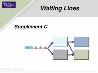
Waiting Lines Supplement C
Waiting Lines • Waiting line: One or more “customers” waiting for service. • Customer population: An input that generates potential customers. • Service facility: A person (or crew), a machine (or group of machines), or both, necessary to perform the service for the customer. • Priority rule: A rule that selects the next customer to be served by the service facility. • Service system: The number of lines and the arrangement of the facilities.
Customer population Service system Served customers Waiting line Service facilities Priority rule Waiting Line ModelsBasic Elements
Service facilities Single line Service facilities Multiple lines © 2007 Pearson Education Waiting Line Arrangements
Service Facility Arrangements Channel:One or more facilities required to perform a given service. Phase: A single step in providing a service. Priority rule: The policy that determines which customer to serve next.
Service facility Service Facility Arrangements Single channel, single phase
Service facility 1 Service facility 2 Service Facility Arrangements Single channel, multiple phase
Service facility 1 Service facility 2 Service Facility Arrangements Multiple channel, single phase
Service facility 1 Service facility 3 Service facility 4 Service facility 2 Service Facility Arrangements Multiple channel, multiple phase
Routing for : 1–2–4 Routing for : 2–4–3 Routing for : 3–2–1–4 Service facility 1 Service facility 2 Service facility 3 Service facility 4 Service Facility Arrangements Mixed Arrangement
Priority Rule • The priority rule determines which customer to serve next. • Most service systems use the first-come, first-serve (FCFS) rule. Other priority rules include: • Earliest promised due date (EDD) • Customer with the shortest expected processing time (SPT) • Preemptive discipline: A rule that allows a customer of higher priority to interrupt the service or another customer.
(T)n n! Pn = e-T [2(1)]4 4! 16 24 P4 = e-2 = 0.090 P4 = e-2(1) Probability DistributionsArrival Times Customer Arrivalsare usually random and can be described by a Poisson distribution. Probability that n customers will arrive… Mean =T Variance =T Example C.1 Arrival rate = 2/hour Probability that 4 customers will arrive… Interarrival times: The time between customer arrivals.
P(t ≤ 0.167 hr) = 1 – e-3(0.167) = 1 – 0.61 = 0.39 Probability DistributionsService time • The exponential distribution describes the probability that the service time will be no more than T time periods. μ= average number of customers completing service per periodt = service time of the customer T= target service time P(t ≤T) = 1 – e-T Mean =1/Variance =(1/)2 Example C.2 If the customer service rate is three per hour, what is the probability that a customer requires less than 10 minutes of service?
Operating Characteristics • Line Length: Number of customers in line. • Number of Customers in System: Includes customers in line and being serviced. • Waiting Time in Line: Waiting for service to begin. • Total Time in System: Elapsed time between entering the line and exiting the system. • Service Facility Utilization: Reflects the percentage of time servers are busy.
Single-ServerModel • The simplest waiting line model involves a single server and a single line of customers. • Assumptions: • The customer population is infinite and patient. • The customers arrive according to a Poisson distribution, with a mean arrival rate of • The service distribution is exponential with a mean service rate of • The mean service rate exceeds the mean arrival rate. • Customers are served on a first-come, first-served basis. • The length of the waiting line is unlimited.
Single-ServerModel l m = Average utilization of the system = l m – l L= Average number of customers in the service system = 1 m – l W= Average time spent in the system, including service = Rn= Probability that n customers are in the system =(1 –r)rn Lq= Average number of customers in the waiting line =L Wq= Average waiting time in line =W
l m Utilization = = = = 0.857, or 85.7% 30 35 – 30 30 35 Average number in system = L = = 6 customers 1 35 – 30 Average time in system = W = = 0.20 hour, or 12 minutes Single-Channel, Single-Phase System Example C.3 Arrival rate (l= 30/hour, Service rate (m = 35/hour Average number in line = Lq = 0.857(6) = 5.14 customers Average time in line = Wq= 0.857(0.20) = 0.17 hour, or 10.28 minutes
Single-Channel, Single-Phase System Arrival rate (l= 30/hour Service rate (m = 35/hour
Multiple-Channel, Single-Phase System • With the multiple-server model, customers form a single line and choose one of s servers when one is available. • The service system has only one phase. • There are s identical servers. • The service distribution for each is exponential. • Mean service time is 1/m • The service rate (s exceeds the arrival rate ().
Multiple-Server Model Example C.5 • American Parcel Service is concerned about the amount of time the company’s trucks are idle, waiting to be unloaded. • The terminal operates with four unloading bays. Each bay requires a crew of two employees, and each crew costs $30/hr. • The estimated cost of an idle truck is $50/hr. Trucks arrive at an average rate of three per hour, according to a Poisson distribution. • Unloading a truck averages one hour with exponential service times. • 4 Unloading bays Crew costs $30/hour • 2 Employees/crew Idle truck costs $50/hour • Arrival rate = 3/hour Service time = 1 hour
= 0.75 3 1(4) Utilization = r = 0= [∑ + ( )]-1 (3/1)n n! 1 1 – 0.75 (3/1)4 4! = 0.0377 0.0377(3/1)4(0.75) 4!(1 – 0.75)2 0(l/m)sr s!(1 – r)2 = 1.53 trucks Average trucks in line = Lq = = 1.53 3 Lq l = = 0.51 hours Average time in line = Wq = 1 1 1 m = 3(1.51) = 1.51 hours = 4.53 trucks Average trucks in system = L = lW Average time in system = W = Wq + = 0.51 + © 2007 Pearson Education Multiple-Server Model 4 Unloading bays Crew costs $30/hour 2 Employees/crew Idle truck costs $50/hour Arrival rate = 3/hour Service time = 1 hour
© 2007 Pearson Education Multiple-Server Model 4 Unloading bays Crew costs $30/hour 2 Employees/crew Idle truck costs $50/hour Arrival rate = 3/hour Service time = 1 hour Labor costs: $30(s) = $30(4) = $120.00 Idle truck cost: $50(L) = $50(4.53) = 226.50 Total hourly cost = $346.50
Application C.3 hrs. (or 4.224 minutes)
Little’s Law • Little’s Law relates the number of customers in a waiting-line system to the waiting time of customers. L = W L is the average number of customers in the system. is the customer arrival rate. W is the average time spent in system, including service.
Finite-Source Model • In the finite-source model, the single-server model assumptions are changed so that the customer population is finite, with N potential customers. • If N is greater than 30 customers, then the single-server model with an infinite customer population is adequate.
0 =probability of zero customers[∑()n]–1 N N! (N – n)! n=0 l+m l Lq = Average number of customers in line = N – (1 – 0) m l L = Average number of customers in the system = N – (1 – 0) Finite-Source Model r = Average utilization of the server = 1 – 0 Wq = Average waiting time in line = Lq[(N – L)l]–1 W = Average time in the system = L[(N – L)l]–1
© 2007 Pearson Education Number of robots = 10 Loss/machine hour = $30 Service time = 10 hrs Maintenance cost = $10/hr Time between failures = 200 hrs Example C.6
Finite-Source Model Example C.6 Solution Number of robots = 10 Loss/machine hour = $30 Service time = 10 hrs Maintenance cost = $10/hr Time between failures = 200 hrs Lq = 0.30 robots L = 0.76 robot 0 = 0.538 Wq = 6.43 hours r = 1 – 0.538 = 0.462 W = 16.43 hours Labor cost: ($10/hr)(8 hrs/day)(0.462 utilization) = $ 36.96 Idle robot cost: (0.76 robot)($30/robot hr)(8 hrs/day) = 182.40 Total daily cost = $219.36
Decision Areas for Management • Using waiting-line analysis, management can improve the service system in one or more of the following areas. • Arrival Rates • Number of Service Facilities • Number of Phases • Number of Servers Per Facility • Server Efficiency • Priority Rule • Line Arrangement