Download
1 / 58
680 likes | 1.52k Views
Chap 3 Foundations of Scalar Diffraction Theory. Content. 3.1 Historical introduction 3.2 From a vector to a scalar theory 3.3 Some mathematical preliminaries 3.4 The Kirchhoff formulation of diffraction by a planar screen

E N D
Content • 3.1 Historical introduction • 3.2 From a vector to a scalar theory • 3.3 Some mathematical preliminaries • 3.4 The Kirchhoff formulation of diffraction by a planar screen • 3.5 The Rayleigh-Sommerfeld formulation of diffraction • 3.6 Comparison of the Kirchhoff and Rayleigh-Sommerfeld theories • 3.7 Further discuss of the Huygens-Fresnel principle • 3.8 Generalization to nonmonochromatic waves • 3.9 Diffraction at boundaries • 3.10 The angular spectrum of plane waves
3.1 Historical introduction • While the theory discussed here is sufficiently general to be applied in other field, such as acoustic-wave and radio-wave propagation, the applications of primary concern will be in the realm of physical optics. • To fully understand the properties of optical imaging and data processing system, it is essential that diffraction and the limitation it imposes on system performance be appreciated.
The edge of the aperture is thin enough such that light maybe regarded as unpolarized. In addition the area of the aperture can not be too small. (or be large enough)
Refraction can be defined as the bending of light rays mat takes place when they pass through a region in which there is a gradient of the local velocity of propagation of the wave. • The most common example occurs when the light wave encounters a sharp boundary between two regions having different refractive indices.
The Kirchhoff and Rayleigh-Sommerdeld theories share certain major simplifications and approximations. • Most important light is treated as a scalar phenomenon, neglecting the fundamentally vectorial nature of the electromagnetic fields.
3.2 From a vector to a scalar theory • In the case of diffraction of light by an aperture, the • and field modified only at the edges of the aperture where light interacts with the material which the edges are composed of , and the effects extend over only a few wavelengths into the aperture itself.
1.Wave eq. (in vectorial form) • (from Maxwell’s eq.) • 2. Wave eq. (in scalar forms) • . • 3. Wave eq. (in phasor forms). • Linear, • Homogeneous, • Isotropic, • Nondispersive, • Nonmagnetic.
Where the optical disturbance u(p, t) = • = U(p) e • U(p) = • and represents position variable (i.e. r) • It follow that (called Helmholtz eq.)
In general Huygens (Huygen’s principle) (Young) Fresnel two assumption Kirchhoff (Fresnel-Kirchhoff formula) Fig. 3.1 Huygens’ envelope construction Rayletgh-Summerfled
3.3 Some mathematical preliminaries • 3.3.1 The Helmholtz equation For a monochromatic wave, the scalar field may be written explicitly (3-1) are the amplitude and phase, respectively, of the where A(P) and wave at position P, while v is the optical frequency. If the real disturbance is to represent an optical wave, it must satisfy the scalar wave equation.
The complex function U(P) serves as an adequate description of the disturbance, since the time dependencies known a priori. If (3-1) is substituted in (3-2), it follows that U must obey the time-independent equation. (3-2) (3-3)
3.3.2 Green’s theorem Give U(P), G(p), Let According Gauss’s divergence thm.
Choice of the Green’s func. G(P) Helmholtz eqs. G(P)= (from Huygens-Fresnel principle) ,
3.3.3 The integral thm. of Helmholtz and Kirchhoff The Kirchhoff formulation of the diffraction problem is based on a certain integral theorem which expresses the solution of the homogenous wave equation at an arbitrary point in terms of the values of the solution and its first derivative on an arbitrary closed surface surrounding that point. The problem is to express the optical disturbance at in terms of its values on the surface S. To solve this problem, we follow Kirchhoff in applying Green’s theorem and in choosing as an auxiliary function a unti-amplitude spherical wave expanding about the point (the so-called free space Green’s function).
Within the volume , the disturbance G, being simply an expanding spherical wave, satisfies the Helmholtz equation as
Choice of the adequate volume denoted as satisfying the requirement of Green thm. • The first requirement of Green thm. is that • exist in the volume of integration. b. The second requirement…(see Goodman P.42) are continuous within the volume
(3-4) This result is known as the integral theorem of Helmholtz and Kirchhoff, it plays an important role in the development of the scalar theory of diffraction, for it allows the field at any point to be expressed in terms of the “boundary value” of the wave on any closed surface surrounding that point.
3.4 The Kirchhoff formula of diffraction by a planar screen Fig. 3.3 Kirchhoff formula of diffraction by a plane screen
3.4.1 Application of the integral theorem uniformly bounded As R→
3.4.2 The Kirchhoff boundary conditions Kirchhoff accordingly adopted the following assumptions [162]: 1. Across the surface , the field distribution U and its derivative are exactly the same as they would be in the absence of the screen. 2. Over the portion of that lies in the geometrical shadow of the screen, the filed distribution U and its derivative are identically zero. These conditions are commonly knows as the Kirchhoff boundary conditions.
3.4.3 The Fresnel-Kirchhoff diffraction formula Fig. 3.4 Point-source illumination a plane screen.
Note: (3-5)
(Fowles) (3-6) Let the illumination source be a point source. (3-7)
3.5 The Rayleigh-Sommerfeld formulation diffraction • It is a well-known theorem of potential theory that if a two-dimensional potential function and its normal derivative vanish together along any finite curve segment, then that potential function must vanish over the entire plane. Similarly, if a solution of the three-dimension wave equation vanishes on any finite surface element, it must vanish in all space.
3.5.1 Choice of alternative Green’s function • The conditions for validity of this equation are: • The scalar theory holds. • 2. Both U and G satisfy the homogeneous scalar wave equation. Helmoltz equation) • 3. The Sommerfeld radiation condition is satisfied.
(3-8) (Kirchhoff spherical wavelet) (Sommerfeld choose)
Fig. 3.5 Rayleigh-Sommerfeld formulation of diffraction by a plane screen
(3-9) (refer to eq. (3-5)) Choose Green func.
(3-10) (3-11)
3.5.2 The Rayleigh-Sommerfeld diffraction formula Rayleigh-Sommerfeld diffraction formula (3-12) (3-13) • Fresnel-Kirchhoff diffraction formula (3-14) (3-15)
3.6 Comparison of the Kirchhoff and Rayleigh-Sommerfeld theories Diffraction by a planar screen ∴
Kirchhoff (one singular point) Sommerfeld (multiple singular point)
Scalar diffraction formula (general form) (Sommerfeld radiation condition) 2 (Kirchhoff) 2G (Kirchhoff)
A comparison of the above equations leads us to an interesting and surprising conclusion: the Kirchhoff solution is the arithmetic average of the two Rayleigh-Sommerfeld solution. • In closing it is worth nothing that, in spite of its internal inconsistencies, there is one sense in which the Kirchhoff theory is more general than the Rayleigh-Sommerfeld theory. The latter requires that the diffracting screens be planar, while the former does not.
3.7 Further discussion of the Huygens-Fresnel principle • It expresses the observed field U( ) as a superposition of diverging spherical Huygens-Fresnel wavelet origination from secondary source located at each every point within the aperture . (3-16)
where the impulse response is given explicitly by (3-17)
3.8 Generalization to nonmonochromatic wave (Nonomonochromatic time function) (3-22) For nonmonochromatic light (3-23) where the phasor implies the Fourier transform (FT) of the disturbance with respect to (w, r, t) the temporal frequency .
Note: Free space (nondispersive medium) Monochromatic source
(3-24) (3-25) or Since
Eq. (3-25) becomes or (3-26) V is the velocity of propagation of the disturbance in a medium of refractive index n (v=c/n), and the relation or has been used.
3.9 Diffraction at boundaries • A more physical point-of-view, first qualitatively expressed by Thomas Young in 1802, is to regard the observed field as consisting of a superposition of the incident wave transmitted through the aperture unperturbed, and a diffracted wave originating at the rim of the aperture. The possibility of a new wave origination in the material medium of the rim makes this interpretation a more physical one. • The applicability of a boundary diffraction approach in more general diffraction problems was investigated by Maggi [202] and Rubinowicz [249], who showed that the Kirchhoff diffraction formula can indeed be manipulated to yield a form that is equivalent to Young’s ideas. More recently, Miyamoto and Wolf [250] have extended the theory of boundary diffraction.
3.10 The angular spectrum of plane waves • Objective: • To formulate scalar diffraction theory in a framework that closely resembles the theory of linear, invariant system. • As we shall see, • if the complex field distribution of a monochromatic disturbance is Fourier-analyzed across any plane, the various spatial Fourier components can be identified as plane waves traveling in different directions always from that plane. • The field amplitude at any other point (or across any other parallel plane) can be calculated by adding the contributions of these plane waves, taking due account of the phase shifts they have undergone during propagation.
3.10.1 The angular spectrum and its physical interpretation Let the complex field, across z=0 plane, be represented by U(x, y, 0). Our ultimate objective is to calculate the resulting field U(x, y, z). Temporal freq. Phasor Spatial freq. The Fourier transform of U(x, y, 0), i.e., its spectrum (3-27) And the inverse Fourier transform of its spectrum (3-28)
To give physical meaning to the function in the integrand of the above integral, consider the plane wave Where the phasor
Thus, across the plane z=0, We see that The angular spectrum of the disturbance
3.10.2 Propagation of the angular spectrum Consider the angular spectrum of the disturbance (3-29) (3-30) into the Helmholz eq.
gives (3-31) where and for all true direction cosines. An elementary solution of Eq. (3-31) can be written in the form (3-32)