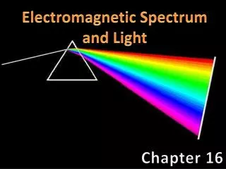
Chap. 3 Electromagnetic Theory and Light
200 likes | 476 Views
Chap. 3 Electromagnetic Theory and Light. Light possesses both wave-particle manifestations. Classical electrodynamics based on Maxwell’s electromagnetic theory unalterably leads to the picture of a continuous transfer of energy by way of electromagnetic waves .

Chap. 3 Electromagnetic Theory and Light
E N D
Presentation Transcript
3- Chap. 3 Electromagnetic Theory and Light Light possesses both wave-particle manifestations. Classical electrodynamics based on Maxwell’s electromagnetic theory unalterably leads to the picture of a continuous transfer of energy by way of electromagnetic waves. Quantum electrodynamics describes electromagnetic interaction and the transport of energy in terms of massless elementary “particles” known as photons, which are localized quanta of energy. One of the basic tenets of quantum mechanics is that both light and material objects each display both wave-particle properties. In physical optics light is treated as an electromagnetic wave. 3.1 Maxwell’s equations The simplest statement of Maxwell’s equations governs the behavior of the electric and magnetic fields in free space. Maxwell’s equations are generalization of experimental results.
3- where and are the permeability and the electric permittivity of free space, respectively. It should be noted that except for a multiplicative scalar, the electric and magnetic fields appears in above equations with a remarkable symmetry. The mathematical symmetry implies a good deal of physical symmetry. Maxwell’s equations tell us that a time-varying magnetic field generates an electric field and a time-varying electric field generates a magnetic field. Maxwell’s equations above can be written in differential form by using following two theorems from vector calculus.
3- By applying theorem (3.5) to Eqs. (3.1) and (3.2) and applying theorem (3.6) to Eqs (3.3) and (3.4), we obtain the following differential equations
3- The consequent equations for free space are in detail as follows:
3- 3.2 Electromagnetic waves Maxwell’s equations for free space can be manipulated into the form of two vector expressions: Taking the curl of Eq. (3.7)
3- The Laplacian, , operates on each component of and , so that the two vector equations (3.18) and (3.19) actually represent a total of 6 scalar equations. One of these expressions, in Cartesian coordinates, is Each component of the electromagnetic field ( ) therefore obeys the scalar differential wave equation provided that If we substitute the values of and into Eq. 3.22, the predicted speed of all electromagnetic waves travelling in free space would then be c= 3 x 10⁸ m/s. This theoretical value was in remarkable agreement with the previously measured speed of light.
3- The experimentally verified transverse character of light should be explained within the context of the electromagnetic theory. To that end, consider the fairly simple case of a plane wave propagating in the positive x-direction and write as . Eq. (3.15) is reduced to For a progressive wave, the solution of (3.23) is Ex=0. So the electric component must be perpendicular to the propagation direction, x. Let’s orient the coordinate axes so that the electric field is parallel to the y-axis: . From Eq. (3.13 III), it follows that This implies that the time-dependent B-field can only have a component in the z-direction. Clearly then, in free space, the plane electromagnetic wave is indeed transverse, as shown in Fig. 3.1. Now let’s write Fig. 3.1 Field configuration in a plane harmonic electromagnetic wave.
3- The associated magnetic field can be found by directly integrating Eq. (3.25), that is, (3.26) Fig. 3.2 Orthogonal harmonic E-field and B_field. Clearly, and have the same time dependence, and are in phase at all points in space. Moreover, and are mutually perpendicular, and their cross-product, , points in the propagation direction, as shown in Fig.3.2. It should be noted that plane waves are not only solutions to Maxwell’s equations. As we saw in the previous chapter, the differential wave equation allows many solutions including spherical waves.
3- 3.3 Energy Energy density, , which is the radiant energy per unit volume, is given by From Eqs. (3.27) and (3.28), we have The amount of energy transported during a unit time and through a unit area perpendicular to the transport direction is (suppose the wave travels through an area of A and with a speed of c and with a time duration of ) The corresponding vector is called Poynting vector: It’s along the wave propagation direction. Its SI unit is watt per square meter ( ).
3- E and B are so closely coupled to each other that we need to deal with only one of them. Using from Eq. 3.26, we can rewrite Eq. 3.30 as The time-averaged value of the magnitude of the Poynting vector, symbolized by , is a measure of the significant quantity known as the irradiance, . Where E0 is the peak magnitude of E. Within a linear, homogeneous, isotropic medium, the expression for the irradiance becomes For a point light source, its irradiance is proportional to . This is well-known inverse-square law. Fig. 3.3 shows that a point source emits electromagnetic waves uniformly in all directions. Let us assume that the energy of the waves is
3- conserved as they spread from the source. Let us also center an imaginary sphere of radius on the source, as shown in Fig. 3.3. If the power of the source is , the irradiance at the sphere must then be Fig. 3.3 A point source emits light isotropically. In Quantum theory, light possesses quantum energy is in unit of angstrom, h is Plank constant.
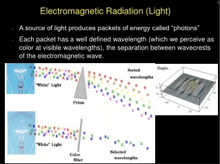
3- 3.4 Electromagnetic-photon spectrum Although all forms of electromagnetic radiation propagate with the same speed in vacuum, they differ in frequency and wavelength. Fig. 3.4 plots the vast electromagnetic spectrum. The frequency range for whole electromagnetic spectrum is from a few Hz to 1022 Hz. The corresponding wavelength range is from many kilometers to 10-14 m. Radiofrequency waves: a few Hz to 109 Hz Microwaves: 109 Hz to about 3 x 10¹¹ Hz. Infrared: 3 x 10¹¹ Hz to 4 x 10¹⁴ Hz. The infrared (IR) is often subdivided into four regions: the near IR (780- 3000 nm), the intermediate IR (3000-6000 nm), the far IR (6000-15,000 nm), and the extreme IR (15,000 nm-1.0 mm). Light: 3.84 x 10¹⁴ to 7.69 x 10¹⁴ Hz. An narrow band of electromagnetic waves could be seen by human eye. Color is not a property of light itself but a manifestation of the electrochemical sensing system-eye, nerves, and brain.
3- Fig. 3.4 Electromagnetic-photon spectrum.
3- Ultraviolet: 8 x 10¹⁴ Hz to 3.4 x 10¹⁶ Hz. X-rays: 2.4 x 10¹⁶ Hz to 5 x 10¹⁹ Hz. Gamma rays: 5 x 10¹⁹ Hz to 2.5 x 1033 Hz. Table 3.1. Frequency and vacuum wavelength ranges for various colors
3- Fig. 3.6 Emission spectrum of GaInP2 semiconductor under excitation of a He-Cd laser.. Fig. 3.5 Spectra of sunlight and the light from a tungsten lamp.
3- 3.5 Light in matter 3.5.1 Dispersion In a homogeneous, isotropic dielectric, the phase velocity of light propagation becomes The ratio of the speed of electromagnetic wave in vacuum to that in matter is known as the absolute index of refraction and is given by For most materials, is generally equal to 1. So, the expression of becomes Actually, n is frequency-dependent, so called dispersion. When a dielectric is subject to an applied electric field E, the internal charge distribution is distorted, which generates electric dipole moment p=Lq, with L the position vector from the negative charge -q to the positive charge q. The dipole moment per unit volume is called the electric polarization P. with
3- Fig. 3.8 shows the dipole formation and a oscillator model for the vibration of electrons under an E-field. The negative electrons are fastened to a stationary positive nucleus. The natural frequency of the spring is with k and m being the spring constant and the electron mass. The force (FE) exerted on an electron of charge q by a harmonic wave E(t) with frequency is Newton’s second law provides the equation of motion with the second term the restoring force. Fig. 3.8 (a) Distortion of the electron cloud in response to an applied E-field. (b) The mechanical oscillator model for an isotropic medium For medium with electron density N the electric polarization P is
3- Eq. (3.44) indicates dispersion. When n>1; When n<1. Fig 3.9 shows dispersion of materials. Fig. 3.9 Index of refraction versus wavelength and frequency for several important optical crystals.
3- 3.5.2 Electric dipole radiation The electric dipole moment oscillates under the electric filed as This oscillation emits radiation. The irradiance (radiated radially outward from the dipole) is given by Fig 3.10 shows the dipole radiation. Notice that the irradiance is inversely proportional to the distance r. The maxima occurs in the direction of . There is no radiation along the dipole axis ( ). Fig. 3.10 Field orientation for an oscillating electric dipole

![Light (Electromagnetic Spectrum) and Telescopes [week 2 and 3]](https://cdn5.slideserve.com/9430149/light-electromagnetic-spectrum-and-telescopes-week-2-and-3-dt.jpg)