Download
1 / 68
880 likes | 2.64k Views
Chap 4 Fresnel and Fraunhofer Diffraction. Content. 4.1 Background 4.2 The Fresnel approximation 4.3 The Fraunhofer approximation 4.4 Examples of Fraunhofer diffraction patterns. 4.1 Background.

E N D
Content 4.1 Background 4.2 The Fresnel approximation 4.3 The Fraunhofer approximation 4.4 Examples of Fraunhofer diffraction patterns
4.1 Background • These approximations, which are commonly made in many fields that deal with wave propagation, will be referred to as Fresnel and Fraunhofer approximations. • In accordance with our view of the wave propagation phenomenon as a “system”, we shall attempt to find approximations that are valid for a wide class of “input” field distributions.
4.1.1 The intensity of a wave field Poynting’s thm. When calculation a diffraction pattern, we will general regard the intensity of the pattern as the quantity we are seeking.
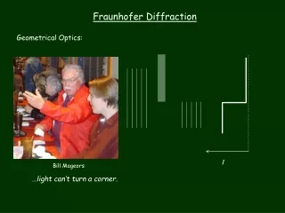
4.1.2 The Huygens-Fresnel principle in rectangular coordinates Before we introducing a series of approximations to the Huygens-Fresnel principle, it will be helping to first state the principle in more explicit from for the case of rectangular coordinates. As shown in Fig. 4.1, the diffracting aperture is assumed to lie in the plane, and is illuminated in the positive z direction. According to Eq. (3-41), the Huygens-Fresnel principle can be stated as (1)
and therefore the Huygens-Fresnel principle can be rewritten (2) (3)
There have been only two approximations in reaching this expression. • One is the approximation inherent in the scalar theory
4.2 Fresnel Diffraction • Recall, the mathematical formulation of the Huygens-Fresnel , the first Rayleigh- Sommerfeld sol. • The Fresnel diffraction means the Fresnel approximation to diffraction between two parallel planes. We can obtain the approximated result. (1)
e (Why?) (wave propagation) wave propagation z Aperture Plane Observation Plane Corresponding to The quadratic-phase exponential with positive phase i.e, ,for z>0
=b Note: The distance from the observation point to an aperture point Using the binominal expansion, we obtain the approximation to
as the term is sufficiently small. The first Rayleigh Sommerfeld sol for diffraction between two parallel planes is then approximated by
( ) , the r01 in denominator of the integrand is supposed to be well approximated by the first term only in the binomial expansion, i.e, • In addition, the aperture points and the observation points are confined to the ( , ) plane and the (x,y) plane ,respectively. ) • Thus, we see
Furthermore, Eq(1) can be rewritten as (2a) • where the convolution kernel is (2b) • Obviously, we may regard the phenomenon of wave propagation as the behavior of a linear system.
Another form of Eq.(1) is found if the term is factored outside the integral signs, it yields (3) which we recognize (aside from the multiplicative factors) to be the Fourier transform of the complex field just to the right of the aperture and a quadratic phase exponential.
We refer to both forms of the result Eqs. (1) and (3), as the Fresnel diffraction integral . When this approximation is valid, the observer is said to be in the region of Fresnel diffraction or equivalently in the near field of the aperture. • Note: • In Eq(1),the quadratic phase exponential in the integrand
do not always have positive phase for z>0 .Its sign depends on the direction of wave propagation. (e.g, diverging of converging spherical waves) In the next subsection ,we deal with the problem of positive or negative phase for the quadratic phase exponent.
4.2.1 Positive vs. Negative Phases Since we treat wave propagation as the behavior of a linear system as described in chap.3 of Goodman), it is important to descries the direction of wave propagation. As a example of description of wave propagation direction, if we move in space in such a way as to intercept portions of a wavefield (of wavefronts ) that were emitted earlier in time.
z t z t z t In the above two illustrations, we assume the wave speed v=zc/tc where zc and tc are both fixed real numbers.
In the case of spherical waves, Diverging spherical wave Converging spherical wave
Consider the wave func. ,where and r >0 and If ,then (Positive phase) implies a diverging spherical wave. Or if
(Negative phase) implies a converging spherical wave. Note: For spherical wave ,we say they are diverging or converging ones instead or saying that they are emitted “earlier in time ” or “later in time”.
“Earlier in time ” Positive phase Specifically, for a time interval tc >0, we see the following relations, The term standing for the time dependence of a traveling wave implies that we have chosen our phasors to rotate in the clockwise direction.
Therefore, we have the following seasonings: • “Earlier in time ” Positive phase (e.g., diverging spherical waves) • “Later in time” Negative phase (e.g., converging spherical waves) Note: “Earlier in time ” means the general statement that if we move in space in such a way as to intercept wavefronts (or portions of a wave-field ) that were emitted earlier in time.
Propagation direction Spatial distribution of wavefronts To describe the direction of wave propagation for plane waves, we cannot use the term diverging or “converging” .Instead .we employ the general statement ,for the following situations.
, (where >0) The phasor of a plane wave, multiplied by the time dependence gives , where We may say that ,if we move in the positive y direction , the argument of the exponential increases in a positive sense, and thus we are moving to a portion of the wave that was emitted earlier in time.
In a similar fashion , we may deal with the situation for Propagation direction
Note: Show that the Huygens-Fresnel principle can be expressed by <pf> Recall the wave field at observation point P0 (1)
For the first Rayleigh –Sommerfeld solution ,the Green func. (2) Note we put the subscript “-”, i.e, G- to signify this kind of Green func. Substituting Eq(2) into Eq.(1) gives
(3) or (4) where the Green func. proposed by Kirchhoff
as or (5) Finally, substituting Eq.(5) into Eq.(4) yields
4.2.2 Accuracy of Fresnel Approximation Recall Fresnel diffraction integral Parabolic wavelet …(4.14) Aperture point (varying withΣ) observation point (fixed) We compare it with the exact formula Spherical wavelet where (or )
since the binomial expansion where The max.approx.error (i.e.,( )max) and the corresponding error of the exponential is maximized at the phase (or approximately 1 radian)
(ξ,η) A sufficient condition for accuracy would be <<1 For example
or This sufficient condition implies that the distance z must be relatively much larger than
Since the binomial expansion (high order term) where we can see that the sufficient condition leads to a sufficient small value of b However, this condition is not necessary. In the following, we will give the next comment that accuracy can be expected for much smaller values of z (i.e., the observation point (x , y) can be located at a relatively much shorter distance to an arbitrary aperture point on the (ξ,η) plane)
We basically malcr use of the argument that for the convolution integral of Eq.(4-14), if the major contribution to the integral comes from points (ξ,η) for which ξ≒x and η≒y, then the values of the HOTs of the expansion become sufficiently small.(That is, as (ξ,η) is close to (x , y) gives a relatively small value Consequently, can be well approximated by . )
In addition it is found that the convolution integral of Eq.(4-14), or where and ,
can be governed by the convolution integral of the function with a second function (i.e., U(ξ,η)) that is smooth and slowly varying for the rang –2 < X < 2 and –2 < Y < 2. Obviously, outside this range, the convolution integral does not yield a significant addition. ( Note For one dimensional case is governed by we can see that is well approximated by
Finally, it appears that the majority of the contribution to the convolution integral for the range -∞ < X < ∞ and -∞ < Y < ∞ or the aperture area Σ comes from that for a square in the (ξ,η) plane with width and centered on the point ξ= x,η= y (i.e., the range –2 < <2 and –2< <2 or < and < ) As a result within the square area, the expansion as well approximated, since is small enough.
From another point of view, since the Fresnel diffraction integral Corresponding square area yields a good approximation to the exact formula where
we may say that for the Fresnel approximation (for the aperture area Σ or the corresponding square area) to give accurate results, it is not necessary that the HOTs of the expansion be small, only that they do not change the value of the Fresnel diffraction integral significantly. Note: From Goodman’s treatment (P.69 70), we see that can well approximate or Where the width of the diffracting aperture is larger than the length of the region –2 < X < 2
For the scaled quadratic-phase exponential of Eqs.(4-14) and Eq.(4-16), the corresponding conclusion is that the majority of the contribution to the convolution integral comes from a square in the (ξ,η) plane, with width and centered on the point (ξ= x ,η= y) • In effect, • When this square lie entirely within the open portion of the aperture, the field observed at distance z is, to a good approximation, what it would be if the aperture were not present. (This is corresponding to the “light” region)
When the square lies entirely behind the obstruction of the aperture, then the observation point lies in a region that is, to a good approximation, dark due to the shadow of the aperture. • When the square bridges the open and obstructed parts of the aperture, then the observed field is in the transition (or gray) region between light and dark. • For the case of a one-dimensional rectangular slit, boundaries among the regions mentioned above can be shown to be parabolas, as illustrated in the following figure.
The light region W – x ≧ , x ≧ 0 W + x ≧ , x <0 Thus, the upper (or lower) boundary between the transition (or gray) region and the light region can be expressed by (or )
4.2.3 The Fresnel approximation and the Angular Spectrum In this subsection, we will see that the Fourier transform of the Fresnel diffraction impression response identical to the transfer func. of the wave propagation phenomenon in the angular spectrum method of analysis, under the condition of small angles. From Eqs.(4-15)and (4-16), We have Where the convolution kernel (or impulse response) is
The FT of the Fresnel diffraction impulse response becomes The integral term can be rewritten a where and